[译]作用于目标识别的选择性搜索

发表于 2019-11-06 更新于 2021-04-11 分类于视觉/vision 阅读次数：

本文字数： 71k 阅读时长 ≈ 2:08

论文下载地址：Selective Search for Object Recognition

摘要

This paper addresses the problem of generating possible object locations for use in object recognition. We introduce Selective Search which combines the strength of both an exhaustive search and segmentation. Like segmentation, we use the image structure to guide our sampling process. Like exhaustive search, we aim to capture all possible object locations. Instead of a single technique to generate possible object locations, we diversify our search and use a variety of complementary image partitionings to deal with as many image conditions as possible. Our Selective Search results in a small set of data-driven, class-independent, high quality locations, yielding 99% recall and a Mean Average Best Overlap of 0.879 at 10,097 locations. The reduced number of locations compared to an exhaustive search enables the use of stronger machine learning techniques and stronger appearance models for object recognition. In this paper we show that our selective search enables the use of the powerful Bag-of-Words model for recognition. The Selective Search software is made publicly available[1].

本文讨论了在目标识别中生成可能的目标位置的问题。我们引入了选择性搜索，它结合了穷举搜索和分割的优点。像分割一样，我们使用图像结构来指导采样过程；像穷举搜索一样，我们的目标是捕获所有可能的目标位置。我们不再使用单一的技术来生成可能的目标位置，而是使搜索多样化，并使用各种互补的图像分割来处理尽可能多的图像条件。选择性搜索算法能够得到一组数据驱动的、与类无关的、高质量的位置，在10097个位置产生99%的召回率和0.879的平均最佳重叠。与穷举搜索相比，位置数目的减少使得能够使用更强的机器学习技术和更强的外观模型进行目标识别。在本文中，我们证明了我们的选择性搜索能够使用强大的单词袋模型进行识别。选择性搜索软件已开源（Matlab版本）

引言

For a long time, objects were sought to be delineated before their identification. This gave rise to segmentation, which aims for a unique partitioning of the image through a generic algorithm, where there is one part for all object silhouettes in the image. Research on this topic has yielded tremendous progress over the past years [3, 6, 13, 26]. But images are intrinsically hierarchical: In Figure 1a the salad and spoons are inside the salad bowl, which in turn stands on the table. Furthermore, depending on the context the term table in this picture can refer to only the wood or include everything on the table. Therefore both the nature of images and the different uses of an object category are hierarchical. This prohibits the unique partitioning of objects for all but the most specific purposes. Hence for most tasks multiple scales in a segmentation are a necessity. This is most naturally addressed by using a hierarchical partitioning, as done for example by Arbelaez et al[3].

很长一段时间以来，人们一直在寻找物体的轮廓，然后才对其进行辨认。这就产生了分割，其目的是通过一种通用算法对图像进行分割，即图像中所有目标轮廓都能得到一个分割图像。近年来，对这一课题的研究取得了巨大的进展。但是图像本质上是分层的：在图1a中，沙拉和勺子在沙拉碗中，而沙拉碗又位于桌子上。此外，根据上下文的不同，本图中的术语表可以仅仅指木材或者包括表上的所有内容。因此，图像的性质和对象类别的不同用途都是层次性的。这禁止对对象进行唯一的分割，但仅限于最特定的用途。因此，对于大多数任务来说，在一个分段中使用多个尺度是必要的。最自然的解决方法是使用分层分区，如Arbelaez等人所做的那样

Besides that a segmentation should be hierarchical, a generic solution for segmentation using a single strategy may not exist at all. There are many conflicting reasons why a region should be grouped together: In Figure 1b the cats can be separated using colour, but their texture is the same. Conversely, in Figure 1c the chameleon is similar to its surrounding leaves in terms of colour, yet its texture differs. Finally, in Figure 1d, the wheels are wildly different from the car in terms of both colour and texture, yet are enclosed by the car. Individual visual features therefore cannot resolve the ambiguity of segmentation.

此外，分割也应该是分层的，使用单个策略进行分割的通用解决方案可能根本不存在。将一个区域组合在一起有许多相互矛盾的原因：在图1b中，猫可以用颜色分开，但它们的纹理是相同的。相反，在图1c中，变色龙的颜色与其周围的叶子相似，但其纹理不同。最后，在图1d中，车轮在颜色和质地上与汽车有着天壤之别，但却被汽车所包围因此，单个视觉特征无法解决分割的模糊性

And, finally, there is a more fundamental problem. Regions with very different characteristics, such as a face over a sweater, can only be combined into one object after it has been established that the object at hand is a human. Hence without prior recognition it is hard to decide that a face and a sweater are part of one object[29].

最后还有一个更根本的问题。具有非常不同特征的区域，例如毛衣上的脸，只有在确定旁边的物体是人之后，才能组合成一个物体。因此，如果没有事先的识别，很难确定一张脸和一件毛衣是一个物体的一部分

This has led to the opposite of the traditional approach: to do localisation through the identification of an object. This recent approach in object recognition has made enormous progress in less than a decade [8, 12, 16, 35]. With an appearance model learned from examples, an exhaustive search is performed where every location within the image is examined as to not miss any potential object location [8, 12, 16, 35].

这导致了与传统方法相反的情况：通过识别对象来进行本地化。最近这种目标识别方法在不到十年的时间里取得了巨大的进步。通过从样本中学习得到外观模型，执行穷举搜索以检查图像中的每个位置，确保不会遗漏任何潜在的对象位置

However, the exhaustive search itself has several drawbacks. Searching every possible location is computationally infeasible. The search space has to be reduced by using a regular grid, fixed scales, and fixed aspect ratios. In most cases the number of locations to visit remains huge, so much that alternative restrictions need to be imposed. The classifier is simplified and the appearance model needs to be fast. Furthermore, a uniform sampling yields many boxes for which it is immediately clear that they are not supportive of an object. Rather then sampling locations blindly using an exhaustive search, a key question is: Can we steer the sampling by a data-driven analysis?

然而，穷举搜索本身有几个缺点。因为搜索每个可能的位置在计算上是不可行的，所以必须通过使用规则网格、固定比例和固定纵横比来减少搜索空间。在大多数情况下可能的位置仍然很多，以至于需要实施其他限制。该方法需要简化分类器结构以快速建立外观模型。此外，均匀采样会产生许多框，很明显它们无法识别具体目标。如何不再盲目地使用穷举搜索进行采样，关键问题是：我们能否通过数据驱动的分析来控制采样？

In this paper, we aim to combine the best of the intuitions of segmentation and exhaustive search and propose a data-driven selective search. Inspired by bottom-up segmentation, we aim to exploit the structure of the image to generate object locations. Inspired by exhaustive search, we aim to capture all possible object locations. Therefore, instead of using a single sampling technique, we aim to diversify the sampling techniques to account for as many image conditions as possible. Specifically, we use a data-driven grouping-based strategy where we increase diversity by using a variety of complementary grouping criteria and a variety of complementary colour spaces with different invariance properties. The set of locations is obtained by combining the locations of these complementary partitionings. Our goal is to generate a class-independent, data-driven, selective search strategy that generates a small set of high-quality object locations.

在本文中，我们的目标是结合分割的直观性和穷举搜索，提出一个数据驱动的选择性搜索算法。受自底向上分割的启发，我们的目标是利用图像的结构来生成目标位置；受穷举搜索的启发，我们的目标是捕获所有可能的目标位置。因此，不是使用单一的采样技术，而是使采样技术多样化，以尽可能多地考虑图像条件。具体来说，我们使用基于数据驱动的分组策略，通过使用各种互补分组准则和具有不同不变性的各种互补颜色空间来增加多样性。通过组合这些互补分区的位置来获得位置集。我们的目标是生成一个独立于类的、数据驱动的、有选择的搜索策略，该策略生成一小组高质量的对象位置

Our application domain of selective search is object recognition. We therefore evaluate on the most commonly used dataset for this purpose, the Pascal VOC detection challenge which consists of 20 object classes. The size of this dataset yields computational constraints for our selective search. Furthermore, the use of this dataset means that the quality of locations is mainly evaluated in terms of bounding boxes. However, our selective search applies to regions as well and is also applicable to concepts such as "grass".

选择性搜索的应用领域是目标识别。因此，我们评估了最常用的数据集，Pascal VOC检测挑战，包括20个对象类。这个数据集的大小为我们的选择性搜索产生了计算约束。此外，使用该数据集意味着位置的质量主要根据边界框来评估。然而，选择性搜索也适用于"草"等概念的区域分割

In this paper we propose selective search for object recognition. Our main research questions are: (1) What are good diversification strategies for adapting segmentation as a selective search strategy? (2) How effective is selective search in creating a small set of high-quality locations within an image? (3) Can we use selective search to employ more powerful classifiers and appearance models for object recognition?

本文中，我们提出作用于目标识别的选择性搜索算法。主要研究问题是:(1) 什么样的多样化策略可以作为选择性搜索策略来适应分割？(2) 选择性搜索在图像中创建一小部分高质量位置的效果如何？(3) 我们可以使用选择性搜索部署更强大的分类器和外观模型来进行对象识别吗？

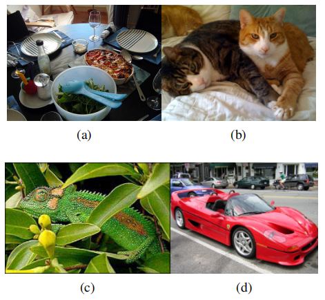
Figure 1: There is a high variety of reasons that an image region forms an object. In (b) the cats can be distinguished by colour, not texture. In (c) the chameleon can be distinguished from the surrounding leaves by texture, not colour. In (d) the wheels can be part of the car because they are enclosed, not because they are similar in texture or colour. Therefore, to find objects in a structured way it is necessary to use a variety of diverse strategies. Furthermore, an image is intrinsically hierarchical as there is no single scale for which the complete table, salad bowl, and salad spoon can be found in (a).

图1：图像区域形成目标的原因多种多样。在（b）中的猫可以用颜色而不是质地来区分。在（c）中的变色龙可以区别于周围叶子的纹理，而不是颜色。在（d）中，车轮可以是汽车的一部分，因为它们是封闭的而不是因为它们的质地或颜色相似。因此，要以结构化的方式找到对象，必须使用多种多样的策略。此外，图像本质上是分层的，因为在（a）中找不到完整的桌子、沙拉碗和沙拉勺

选择性搜索

In this section we detail our selective search algorithm for object recognition and present a variety of diversification strategies to deal with as many image conditions as possible. A selective search algorithm is subject to the following design considerations:

在这一节中，我们详细介绍了目标识别的选择性搜索算法，并提出了各种各样的策略来处理尽可能多的图像条件。选择性搜索算法需要考虑以下设计因素：

Capture All Scales. Objects can occur at any scale within the image. Furthermore, some objects have less clear boundaries then other objects. Therefore, in selective search all object scales have to be taken into account, as illustrated in Figure 2. This is most naturally achieved by using an hierarchical algorithm.

捕获全尺度。对象可以在图像中以任何比例出现。此外，一些对象的边界比其他对象的边界更不清晰。因此，在选择性搜索中必须考虑所有对象比例，如图2所示。最自然的方法是使用分层算法

Diversification. There is no single optimal strategy to group regions together. As observed earlier in Figure 1, regions may form an object because of only colour, only texture, or because parts are enclosed. Furthermore, lighting conditions such as shading and the colour of the light may influence how regions form an object. Therefore instead of a single strategy which works well in most cases, we want to have a diverse set of strategies to deal with all cases.

多元化。没有一个单一的最优策略可以将区域组合在一起。如图1所示，区域可以形成一个对象，因为只有颜色，只有纹理，或因为部分是封闭的。此外，诸如阴影和光的颜色等照明条件可能影响区域形成对象的方式。因此，我们希望有一套不同的策略来处理所有的情况，而不是一个在大多数情况下都很有效的单一策略

Fast to Compute. The goal of selective search is to yield a set of possible object locations for use in a practical object recognition framework. The creation of this set should not become a computational bottleneck, hence our algorithm should be reasonably fast.

快速计算。选择性搜索的目的是产生一组可能的目标位置，用于实际的目标识别框架。这个集合的创建不应该成为计算瓶颈，因此我们的算法应该相当快

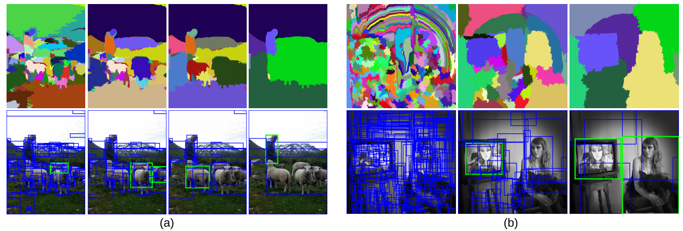
Figure 2: Two examples of our selective search showing the necessity of different scales. On the left we find many objects at different scales. On the right we necessarily find the objects at different scales as the girl is contained by the tv.

图2：选择性搜索的两个例子显示了不同尺度的必要性。在左图中发现了许多不同比例的物体。在右图中能找到不同尺度的物体，即使女孩出现在电视中

按层次分组的选择性搜索

We take a hierarchical grouping algorithm to form the basis of our selective search. Bottom-up grouping is a popular approach to segmentation [6, 13], hence we adapt it for selective search. Because the process of grouping itself is hierarchical, we can naturally generate locations at all scales by continuing the grouping process until the whole image becomes a single region. This satisfies the condition of capturing all scales.

我们采用分层分组算法作为选择性搜索的基础。自底向上分组是一种流行的分割方法[6，13]，因此我们将其用于选择性搜索。由于分组过程本身是分层的，所以我们可以通过继续分组过程自然地在所有尺度上生成位置，直到整个图像变成一个区域。这满足捕获所有尺度的条件

As regions can yield richer information than pixels, we want to use region-based features whenever possible. To get a set of small starting regions which ideally do not span multiple objects, we use the fast method of Felzenszwalb and Huttenlocher [13], which [3] found well-suited for such purpose.

由于区域可以产生比像素更丰富的信息，因此我们希望尽可能使用基于区域的特征。为了得到一组理想情况下不跨越多个对象的小起始区域，我们使用了Felzenszwalb和Huttenlocher[13]的快速方法，这种方法在文章[3]中已证明非常符合这样的要求

Our grouping procedure now works as follows. We first use [13] to create initial regions. Then we use a greedy algorithm to iteratively group regions together: First the similarities between all neighbouring regions are calculated. The two most similar regions are grouped together, and new similarities are calculated between the resulting region and its neighbours. The process of grouping the most similar regions is repeated until the whole image becomes a single region. The general method is detailed in Algorithm 1.

现在我们的分组过程如下，首先使用[13]来创建初始区域。然后利用贪心算法对区域进行迭代分组：首先计算所有相邻区域之间的相似度。将两个最相似的区域组合在一起，并计算结果区域与其相邻区域之间的新相似性。重复组合最相似的区域，直到整个图像变成一个区域为止。方法在算法1中详细说明

Algorithm 1: Hierarchical Grouping Algorithm
Input: (colour)image
Output: Set of object location hypotheses $L$
Obtain initial regions $R={r_{1},...,r_{n}}$ using [13]
Initialise similarity set $S=$
foreach Neighbouring region pair $(r_{i},r_{j})$ do Calculate similarity $s(r_{i},r_{j})$ $S = S \cup s(r_{i},r_{j})$
while $S$ do Get highest similarity $s(r_{i},r_{j}) = max(S)$ Merge corresponding regions $r_{t} = r_{i} \cup r_{j}$ Remove similarities regarding $r_{i}: S = S\setminus s(r_{i},r_{\ast })$ Remove similarities regarding $r_{i}: S = S\setminus s(r_{\ast }, r_{j})$ Calculate similarity set $S_{t}$ between $r_{t}$ and its neighbours $S = S \cup S_{t}$
$R = R \cup r_{t}$
Extract object location boxes $L$ from all regions in $R$

算法1：分层分组算法
输入：（彩色）图像
输出：一组目标定位假设$L$
使用论文[13]的方法获取初始区域$R={r_{1},...,r_{n}}$
初始化相似集$S=$（空集）
foreach 相邻区域对$(r_{i},r_{j})$ do
- 计算相似度$s(r_{i},r_{j})$
- $S = S \cup s(r_{i},r_{j})$（并集）
while $S$ do
- 获取最高相似度$s(r_{i},r_{j}) = max(S)$
- 合并相应的区域$r_{t} = r_{i} \cup r_{j}$
- 移除与$r_{i}$相关的相似度：$S = S\setminus s(r_{i},r_{\ast })$
- 移除与$r_{j}$相关的相似度：$S = S\setminus s(r_{\ast },r_{j})$
- 计算新区域$r_{t}$与周围区域的相似集$S_{t}$
- $S = S \cup S_{t}$ （每次操作后相似集$S$都会减少，最后仅包含一个区域，就是整个图像）
- $R = R \cup r_{t}$（每次操作后区域集R均会增加，自底而上不断的组合可能的目标位置）
从$R$中的所有区域提取目标位置框$L$

For the similarity $s(r_{i},r_{j})$ between region $r_{i}$ and $r_{j}$ we want a variety of complementary measures under the constraint that they are fast to compute. In effect, this means that the similarities should be based on features that can be propagated through the hierarchy, i.e. when merging region $r_{i}$ and $r_{j}$ into $r_{t}$, the features of region $r_{t}$ need to be calculated from the features of $r_{i}$ and $r_{j}$ without accessing the image pixels.

对于区域$r_{i}$和区域$r_{j}$之间的相似性$s(r_{i}，r_{j})$，我们希望在它们快速计算的约束下仍有各种互补措施。实际上，这意味着相似性应该基于可以通过层次结构传播的特征，也就是说，当将区域$r_{i}$和$r_{j}$合并为$r_{t}$时，区域$r_{t}$的特征可以在不访问图像像素的情况下从$r_{i}$和$r_{j}$的特征中计算出来

多元化策略

The second design criterion for selective search is to diversify the sampling and create a set of complementary strategies whose locations are combined afterwards. We diversify our selective search (1) by using a variety of colour spaces with different invariance properties, (2) by using different similarity measures $s_{ij}$, and (3) by varying our starting regions.

选择性搜索的第二个设计准则是使采样多样化，并创建一组互补策略，然后将其位置组合起来。选择性搜索多样化策略如下：（1）使用具有不同不变性的各种颜色空间；（2）使用不同的相似性度量$s_{ij}$，以及（3）改变我们的起始区域

Complementary Colour Spaces. We want to account for different scene and lighting conditions. Therefore we perform our hierarchical grouping algorithm in a variety of colour spaces with a range of invariance properties. Specifically, we the following colour spaces with an increasing degree of invariance: (1) RGB, (2) the intensity (grey-scale image) I, (3) Lab, (4) the rg channels of normalized RGB plus intensity denoted as rgI, (5) HSV, (6) normalized RGB denoted as rgb, (7) C [14] which is an opponent colour space where intensity is divided out, and finally (8) the Hue channel H from HSV. The specific invariance properties are listed in Table 1.

互补颜色空间。我们要考虑不同的场景和照明条件。因此，我们在一系列具有不变性的颜色空间中执行我们的分层分组算法。具体地说，我们用一个不断增加的不变性度来表示下列颜色空间：（1）RGB，（2）强度（灰度图像）I，（3）Lab，（4）归一化RGB的rg通道加上强度，表示为rgI，（5）HSV，（6）归一化RGB，表示为rgb，（7）C[14]是与强度的颜色空间，最后（8）HSV的色调通道H。表1列出了具体的不变性属性

Of course, for images that are black and white a change of colour space has little impact on the final outcome of the algorithm. For these images we rely on the other diversification methods for ensuring good object locations.

当然，对于黑白图像，颜色空间的变化对算法的最终结果影响不大。对于这些图像，我们依赖其他多样化的方法来确保良好的目标位置

In this paper we always use a single colour space throughout the algorithm, meaning that both the initial grouping algorithm of [13] and our subsequent grouping algorithm are performed in this colour space.

在本文中，我们在整个算法中始终使用单一颜色空间，这意味着[13]的初始分组算法和我们的后续分组算法都在该颜色空间中执行

Table 1: The invariance properties of both the individual colour channels and the colour spaces used in this paper, sorted by degree of invariance. A "+/-" means partial invariance. A fraction 1/3 means that one of the three colour channels is invariant to said property.

表一：本文中使用的单个颜色通道和颜色空间的不变性，按不变性程度排序。"+/-"表示部分不变性。分数1/3表示三个颜色通道中的一个对所述属性不变

Complementary Similarity Measures. We define four complementary, fast-to-compute similarity measures. These measures are all in range [0,1] which facilitates combinations of these measures.

互补相似度量。我们定义了四个互补的、快速计算相似度的度量。这些测量值都在[0,1]范围内，这有助于这些测量值的组合

$S_{colour}(r_{i}, r_{j})$ measures colour similarity. Specifically, for each region we obtain one-dimensional colour histograms for each colour channel using 25 bins, which we found to work well. This leads to a colour histogram $C_{i}={c_{i}^{1}, ..., c_{i}^{n}}$ for each region $r_{i}$ with dimensionality $n = 75$ when three colour channels are used. The colour histograms are normalised using the $L_{1}$ norm. Similarity is measured using the histogram intersection:

$S_{colour}(r_{i}, r_{j})$ 测量颜色相似性。具体来说，对于每个区域，我们使用25个bin获得每个颜色通道的一维颜色直方图，我们发现效果很好。所以三通道彩色直方图$C_{i}={C_{i}^{1},...,C_{i}^{n}}$的维度为$n=75$。彩色直方图使用$L_{1}$标准化。相似性通过直方图相交来测量：

\[ S_{colour}(r_{i}, r_{j})=\sum_{k=1}^{n} \min(c_{i}^{k}, c_{j}^{k}) \]

The colour histograms can be efficiently propagated through the hierarchy by

颜色直方图可以通过以下方式在层次结构中有效传播

\[ C_{t}=\frac{size(r_{i})\times C_{i} + size(r_{j})\times C_{j}}{size(r_{i}) + size(r_{j})} \]

The size of a resulting region is simply the sum of its constituents: $size(r_{t}) = size(r_{i})+size(r_{j})$

结果区域的大小只是其成分的总和: $size(r_{t}) = size(r_{i})+size(r_{j})$

$S_{texture}(r_{i}, r_{j})$ measures texture similarity. We represent texture using fast SIFT-like measurements as SIFT itself works well for material recognition [20]. We take Gaussian derivatives in eight orientations using $σ = 1$ for each colour channel. For each orientation for each colour channel we extract a histogram using a bin size of 10. This leads to a texture histogram $T_{i} = {t_{i}^{1}, ..., t_{i}^{n}}$ for each region $r_{i}$ with dimensionality $n = 240$ when three colour channels are used. Texture histograms are normalised using the $L_{1}$ norm. Similarity is measured using histogram intersection:

$S_{texture}(r_{i}, r_{j})$ 测量纹理相似性。我们使用快速的类SIFT测量来表示纹理，因为SIFT本身对材料识别很有效[20]。我们采用八个方向的高斯导数，每个颜色通道使用$σ=1$。对于每个颜色通道的每个方向，我们使用10个bin来提取直方图。所以三通道区域$r_{i}$的纹理直方图$T{i}={T{i}^{1}，…，T{i}^{n}}$的维度为$n=240$。纹理直方图使用$L_{1}$进行规范化。相似性通过直方图相交来测量：

\[ S_{texture}(r_{i}, r_{j}) = \sum_{k=1}^{n} \min (t_{i}^{k}, t_{j}^{k}) \]

Texture histograms are efficiently propagated through the hierarchy in the same way as the colour histograms.

纹理直方图在层次结构中的传播方式与颜色直方图相同

$S_{size}(r_{i}, r_{j})$ encourages small regions to merge early. This forces regions in $S$, i.e. regions which have not yet been merged, to be of similar sizes throughout the algorithm. This is desirable because it ensures that object locations at all scales are created at all parts of the image. For example, it prevents a single region from gobbling up all other regions one by one, yielding all scales only at the location of this growing region and nowhere else. $S_{size}(r_{i},r_{j})$ is defined as the fraction of the image that $r_{i}$ and $r_{j}$ jointly occupy:

$S_{size}(r_{i}, r_{j})$ 鼓励小区域尽早合并。这迫使$S$中的区域（即尚未合并的区域）在整个算法中具有相似的大小。这是可取的，因为它可以确保在图像的所有部分创建所有比例的对象位置（每次分层分组算法能够产生一个假设目标位置）。例如，它防止单个区域一个接一个地吞食所有其他区域，只在这个区域位置附近产生所有候选的目标位置。$S_{size}(r_{i}, r_{j})$定义为$r_{i}$和$r_{j}$共同占用的图像的分数：

\[ S_{size}(r_{i}, r_{j})=1 - \frac{size(r_{i}) + size(r_{j})}{size(im)} \]

where $size(im)$ denotes the size of the image in pixel.

其中$size(im)$表示图像的像素大小

$S_{fill}(r_{i}, r_{j})$ measures how well region $r_{i}$ and $r_{j}$ fit into each other. The idea is to fill gaps: if $r_{i}$ is contained in $r_{j}$ it is logical to merge these first in order to avoid any holes. On the other hand, if $r_{i}$ and $r_{j}$ are hardly touching each other they will likely form a strange region and should not be merged. To keep the measure fast, we use only the size of the regions and of the containing boxes. Specifically, we define $BB_{ij}$ to be the tight bounding box around $r_{i}$ and $r_{j}$. Now $S_{fill}(r_{i},r_{j})$ is the fraction of the image contained in $BB_{ij}$ which is not covered by the regions of $r_{i}$ and $r_{j}$:

$S_{fill}(r_{i}, r_{j})$ 测量区域$r_{i}$和$r_{j}$的匹配程度。理想情况下是两个区域能够填补相互的空白：如果$r_{i}$包含在$r_{j}$中，那么首先合并这两个区域以避免大的空白出现是合乎逻辑的。换句话说，如果$r_{i}$和$r_{j}$几乎不接触在一起，那么他们将形成一个奇怪的区域，不应该被合并。为了保持度量的快速性，我们只使用区域和包含框的大小。具体来说，我们将$BB_{ij}$定义为$r_{i}$和$r_{j}$周围的紧边界框。现在$S_{fill}(r_{i},r_{j})$表示$BB_{ij}$中没有被$r_{i}$和$r_{j}$所覆盖的区域占整个图像的比例：

\[ fill(r_{i},r_{j})=1 - \frac {size(BB_{ij})-size(r_{i})-size(r_{j})}{size(im)} \]

We divide by $size(im)$ for consistency with Equation 4. Note that this measure can be efficiently calculated by keeping track of the bounding boxes around each region, as the bounding box around two regions can be easily derived from these.

$size(im)$表示图像像素个数。请注意，通过跟踪每个区域周围的边界框，可以有效地计算此度量，因为两个区域周围的边界框很容易从中导出。

In this paper, our final similarity measure is a combination of the above four:

在本文中，我们的最终相似性度量是上述四项的组合：

\[ s(r_{i},r_{j})=a_{1}s_{colour}(r_{i},r_{j})+a_{2}s_{texture}(r_{i},r_{j})+a_{d}s_{size}(r_{i},r_{j})+a_{r}s_{fill}(r_{i},r_{j}) \]

where $a_{i}∈{0,1}$ denotes if the similarity measure is used or not. As we aim to diversify our strategies, we do not consider any weighted similarities.

其中$a_{i}$取值为$0$或者$1$，表明是否使用此项相似度度量。由于我们的目标是使我们的战略多样化，我们不考虑任何加权相似性

Complementary Starting Regions. A third diversification strategy is varying the complementary starting regions. To the best of our knowledge, the method of [13] is the fastest, publicly available algorithm that yields high quality starting locations. We could not find any other algorithm with similar computational efficiency so we use only this oversegmentation in this paper. But note that different starting regions are (already) obtained by varying the colour spaces, each which has different invariance properties. Additionally, we vary the threshold parameter $k$ in [13].

互补起始区域。第三个多样化战略是改变互补的起始区域。据我们所知，[13]的方法是最快的、公开可用的算法，能够产生高质量的起始位置。我们找不到任何其他算法具有类似的计算效率，所以本文只使用这种过度分割方法。但是请注意，不同的起始区域是通过改变颜色空间获得的，每个颜色空间具有不同的不变性。此外，我们可以改变文章[13]中的阈值参数$k$以获得不同的起始空间

组合位置

In this paper, we combine the object hypotheses of several variations of our hierarchical grouping algorithm. Ideally, we want to order the object hypotheses in such a way that the locations which are most likely to be an object come first. This enables one to find a good trade-off between the quality and quantity of the resulting object hypothesis set, depending on the computational efficiency of the subsequent feature extraction and classification method.

在本文中，我们结合了我们的分层分组算法的几种变体的目标假设。理想情况下，我们希望对目标假设进行排序，以便最有可能是目标的位置排在第一位。这使得人们能够根据后续特征提取和分类方法的计算效率，在结果目标假设集的质量和数量之间找到一个很好的折衷

We choose to order the combined object hypotheses set based on the order in which the hypotheses were generated in each individual grouping strategy. However, as we combine results from up to 80 different strategies, such order would too heavily emphasize large regions. To prevent this, we include some randomness as follows. Given a grouping strategy $j$, let $r_{i}^{j}$ be the region which is created at position $i$ in the hierarchy, where $i = 1$ represents the top of the hierarchy (whose corresponding region covers the complete image). We now calculate the position value $v_{i}^{j}$ as $RND×i$, where $RND$ is a random number in range [0,1]. The final ranking is obtained by ordering the regions using $v_{i}^{j}$.

根据假设集在每个单独分组策略中的生成顺序来得到最终的假设目标顺序。然而，当我们将多达80种不同策略的结果结合起来时，这种顺序将过于强调大区域。为了防止这种情况，我们增加一些随机性。给定一个分组策略$j$，$r_{i}^{j}$表示在该分组分层计算中第$i$次创建的假设区域，其中$i=1$表示该次分层的顶部（其对应的区域覆盖整个图像）。现在将位置值$v_{i}^{j}$计算为$RND\times i$，其中$RND$是[0,1]范围内的随机数。最后的排名是通过对区域按$v_{i}^{j}$排序获得的

个人解析：

每次子单独的分组策略中都能生成一个假设集，组合这些假设集得到最终的目标假设集
单个假设集的位置都是按从大到小排序，所以使用随机数RND重新排列单个假设集中的假设目标位置

When we use locations in terms of bounding boxes, we first rank all the locations as detailed above. Only afterwards we filter out lower ranked duplicates. This ensures that duplicate boxes have a better chance of obtaining a high rank. This is desirable because if multiple grouping strategies suggest the same box location, it is likely to come from a visually coherent part of the image.

当我们使用边界框中的位置时，我们首先按照上面的详细说明排列所有位置。只有在这之后我们才能过滤出排名较低的重复项。这样可以确保重复框有更好的机会获得高等级。这是可取的，因为如果多个分组策略建议相同的框位置，则它很可能来自图像的视觉连贯部分

个人解析：不同的假设集中可能会提出相同的边界框，通过上述方法打乱假设集的目标位置后再进行过滤

使用选择性搜索进行目标识别

This paper uses the locations generated by our selective search for object recognition. This section details our framework for object recognition.

本文利用选择性搜索产生的位置进行目标识别。本节详细介绍目标识别框架

Two types of features are dominant in object recognition: histograms of oriented gradients (HOG) [8] and bag-of-words [7, 27]. HOG has been shown to be successful in combination with the partbased model by Felzenszwalb et al. [12]. However, as they use an exhaustive search, HOG features in combination with a linear classifier is the only feasible choice from a computational perspective. In contrast, our selective search enables the use of more expensive and potentially more powerful features. Therefore we use bag-of-words for object recognition [16, 17, 34]. However, we use a more powerful (and expensive) implementation than [16, 17, 34] by employing a variety of colour-SIFT descriptors [32] and a finer spatial pyramid division [18].

在对象识别中，两类特征占主导地位：方向梯度直方图（HOG）[8]和单词包[7，27]。Felzenszwalb等人证明了将HOG与基于部分的模型结合起来是成功的[12]。然而，由于它们使用穷举搜索，从计算角度来看，HOG特征与线性分类器结合是唯一可行的选择。相比之下，我们的选择性搜索能够使用更昂贵和潜在更强大的功能。因此，我们使用单词包进行对象识别[16，17，34]。然而，我们使用比[16，17，34]更强大（和昂贵）的实现，通过使用各种颜色筛选描述符[32]和更精细的空间金字塔分割[18]

Specifically we sample descriptors at each pixel on a single scale (σ = 1.2). Using software from [32], we extract SIFT [21] and two colour SIFTs which were found to be the most sensitive for detecting image structures, Extended OpponentSIFT [31] and RGB-SIFT [32]. We use a visual codebook of size 4,000 and a spatial pyramid with 4 levels using a 1x1, 2x2, 3x3. and 4x4 division. This gives a total feature vector length of 360,000. In image classification, features of this size are already used [25, 37]. Because a spatial pyramid results in a coarser spatial subdivision than the cells which make up a HOG descriptor, our features contain less information about the specific spatial layout of the object. Therefore, HOG is better suited for rigid objects and our features are better suited for deformable object types.

具体来说，我们在单个尺度上对每个像素的描述符进行采样（σ=1.2）。利用文献[32]中的软件，我们提取了SIFT[21]和两个对检测图像结构最敏感的颜色筛：扩展OpponentSIFT[31]和RGB-SIFT[32]。我们使用4000大小的视觉码本和4层空间金字塔，使用1x1、2x2、3x3和4x4分区。这使得特征向量的总长度为360000。在图像分类中，已经使用了这种大小的特征[25，37]。由于空间金字塔比构成HOG描述符的单元产生更粗糙的空间细分，因此我们的特征包含的关于对象的特定空间布局的信息更少。因此，HOG更适合于刚性对象，而我们的特征更适合于可变形对象类型

As classifier we employ a Support Vector Machine with a histogram intersection kernel using the Shogun Toolbox [28]. To apply the trained classifier, we use the fast, approximate classification strategy of [22], which was shown to work well for Bag-of-Words in [30].

作为分类器，我们使用使用Shogun工具箱[28]部署了一个支持向量机和一个直方图相交核。为了应用训练的分类器，我们使用了[22]的快速、近似分类策略，这在[30]中被证明是很好的

Our training procedure is illustrated in Figure 3. The initial positive examples consist of all ground truth object windows. As initial negative examples we select from all object locations generated by our selective search that have an overlap of 20% to 50% with a positive example. To avoid near-duplicate negative examples, a negative example is excluded if it has more than 70% overlap with another negative. To keep the number of initial negatives per class below 20,000, we randomly drop half of the negatives for the classes car, cat, dog and person. Intuitively, this set of examples can be seen as difficult negatives which are close to the positive examples. This means they are close to the decision boundary and are therefore likely to become support vectors even when the complete set of negatives would be considered. Indeed, we found that this selection of training examples gives reasonably good initial classification models.

训练步骤如图3所示。最初的正面例子由所有真值目标窗口组成。作为最初的负样本实例，从选择性搜索生成的所有目标位置中选择与正样本实例重叠20%到50%的位置。为了避免近似重复的负样本，如果负样本实例与另一负样本实例的重叠超过70%，则将其排除。为了使每类的初始负样本数保持在20000个以下，我们随机舍弃一半的汽车、猫、狗和人的负样本。直觉上，这组示例可以被看作是很接近于正样本的负样本。这意味着它们接近于决策边界，因此，即使考虑到全套否定，它们也很可能成为支持向量。事实上，我们发现这种训练示例的选择提供了相当好的初始分类模型。

Then we enter a retraining phase to iteratively add hard negative examples (e.g. [12]): We apply the learned models to the training set using the locations generated by our selective search. For each negative image we add the highest scoring location. As our initial training set already yields good models, our models converge in only two iterations.

然后我们进入一个再训练阶段，迭代添加新的负样本（例如[12]）：使用选择性搜索生成的位置将学习到的模型应用到训练集。对于每一张负样本图片，我们都会加上得分最高的位置。由于我们的初始训练集已经产生了好的模型，我们的模型只在两次迭代中收敛

For the test set, the final model is applied to all locations generated by our selective search. The windows are sorted by classifier score while windows which have more than 30% overlap with a higher scoring window are considered near-duplicates and are removed.

对于测试集，最终模型将应用于我们的选择性搜索生成的所有位置。窗口按分类器得分排序，与得分较高的窗口重叠超过30%的窗口被视为接近重复项并被删除

Figure 3: The training procedure of our object recognition pipeline. As positive learning examples we use the ground truth. As negatives we use examples that have a 20-50% overlap with the positive examples. We iteratively add hard negatives using a retraining phase.

图3：目标识别训练过程。通过标注数据作为正样本；使用与正样本有20-50%的重叠的数据作为负样本。在继续训练阶段反复添加错误分类样本

评价

In this section we evaluate the quality of our selective search. We divide our experiments in four parts, each spanning a separate subsection:

在本节中，我们将评估选择性搜索的质量。把实验分成四个部分，每个部分跨越一个单独的子章节：

Diversification Strategies. We experiment with a variety of colour spaces, similarity measures, and thresholds of the initial regions, all which were detailed in Section 3.2. We seek a trade-off between the number of generated object hypotheses, computation time, and the quality of object locations. We do this in terms of bounding boxes. This results in a selection of complementary techniques which together serve as our final selective search method.

多样化策略。使用各种颜色空间、相似性度量和初始区域阈值进行实验，所有这些都在第3.2节中详细说明。寻求在生成的目标假设数量、计算时间和目标位置质量之间的权衡。我们是通过边界框完成的。这导致了互补技术的选择，这些技术共同作为我们的最终选择搜索方法

Quality of Locations. We test the quality of the object location hypotheses resulting from the selective search.

位置质量。我们测试了由选择性搜索产生的目标定位假设的质量

Object Recognition. We use the locations of our selective search in the Object Recognition framework detailed in Section 4. We evaluate performance on the Pascal VOC detection challenge.

目标识别。我们在第4节详述的目标识别框架中使用选择性搜索得到的位置。在Pascal VOC检测挑战中评估性能

An upper bound of location quality. We investigate how well our object recognition framework performs when using an object hypothesis set of "perfect" quality. How does this compare to the locations that our selective search generates?

定位质量的上限。我们研究了目标识别框架在使用“完美”质量的对象假设集时的性能，这与选择性搜索生成的位置相比如何？

To evaluate the quality of our object hypotheses we define the Average Best Overlap (ABO) and Mean Average Best Overlap (MABO) scores, which slightly generalises the measure used in [9]. To calculate the Average Best Overlap for a specific class $c$, we calculate the best overlap between each ground truth annotation $g_{i}^{c} ∈ G^{c}$ and the object hypotheses $L$ generated for the corresponding image, and average:

为了评估目标假设的质量，定义了平均最佳重叠（ABO）和均值平均最佳重叠（MABO）分数，这稍微概括了[9]中使用的测量方法。为了计算特定类$c$的平均最佳重叠，我们计算每个正确标注注释$g_{i}^{c}∈G^{c}$与为相应图像生成的对象假设$L$之间的最佳重叠，并且平均：

\[ ABO=\frac {1}{|C^{c}|} \sum_{g_{i}^{c}\in G^{c}} \max_{l_{j}\in L} Overlap(g_{i}^{c}, l_{j}) \]

The Overlap score is taken from [11] and measures the area of the intersection of two regions divided by its union:

重叠分数公式取自[11]，测量两个区域的相交面积除以其并集：

\[ Overlap(g_{i}^{c}, l_{j})=\frac {area(g_{i}^{c})\cap area(1_{j})}{area(g_{i}^{c})\cup area(1_{j})} \]

Analogously to Average Precision and Mean Average Precision, Mean Average Best Overlap is now defined as the mean ABO over all classes.

与平均精度和平均精度均值类似，均值平均最佳重叠现在定义为所有类的均值ABO

Other work often uses the recall derived from the Pascal Overlap Criterion to measure the quality of the boxes [1, 16, 34]. This criterion considers an object to be found when the Overlap of Equation 8 is larger than 0.5. However, in many of our experiments we obtain a recall between 95% and 100% for most classes, making this measure too insensitive for this paper. However, we do report this measure when comparing with other work.

其他的工作经常使用来自Pascal重叠标准来测量框的质量[1，16，34]。当上式的重叠度大于0.5时，该准则认为找到了一个物体。然而，在我们的许多实验中，对于大多数类，我们获得了95%到100%的召回率，这使得本文对这个度量太不敏感了。但是在与其他工作进行比较时，我们还是报告了这一结果

To avoid overfitting, we perform the diversification strategies experiments on the Pascal VOC 2007 TRAIN+VAL set. Other experiments are done on the Pascal VOC 2007 TEST set. Additionally, our object recognition system is benchmarked on the Pascal VOC 2010 detection challenge, using the independent evaluation server.

为避免过拟合，我们在Pascal VOC 2007 TRAIN+VAL集上进行了多样化策略实验。此外，我们的目标识别系统以帕斯卡VOC 2010检测挑战作为基准，使用独立的评估服务器

多样化策略

In this section we evaluate a variety of strategies to obtain good quality object location hypotheses using a reasonable number of boxes computed within a reasonable amount of time.

在这一部分中，我们评估了各种策略，以使用在合理时间内计算出的合理数量的框来获得高质量的目标位置假设

平面 vs. 分层

In the description of our method we claim that using a full hierarchy is more natural than using multiple flat partitionings by changing a threshold. In this section we test whether the use of a hierarchy also leads to better results. We therefore compare the use of [13] with multiple thresholds against our proposed algorithm. Specifically, we perform both strategies in RGB colour space. For [13], we vary the threshold from k = 50 to k = 1000 in steps of 50. This range captures both small and large regions. Additionally, as a special type of threshold, we include the whole image as an object location because quite a few images contain a single large object only. Furthermore, we also take a coarser range from k = 50 to k = 950 in steps of 100. For our algorithm, to create initial regions we use a threshold of k = 50, ensuring that both strategies have an identical smallest scale. Additionally, as we generate fewer regions, we combine results using k = 50 and k = 100. As similarity measure S we use the addition of all four similarities as defined in Equation 6. Results are in table 2.

在我们方法的描述中，我们声称使用完整的层次结构比通过更改阈值使用多个平面分区更自然。在本节中，我们将测试层次结构的使用是否也会导致更好的结果。因此，我们将[13]的多阈值使用与我们提出的算法进行了比较。具体来说，我们在RGB颜色空间中执行这两种策略。对于[13]，我们将阈值从k=50变为k=1000，步长为50。这一范围涵盖了小区域和大区域。另外，作为一种特殊的阈值类型，我们将整个图像作为一个对象位置，因为很多图像只包含一个大对象。此外，我们还采取了一个较粗的范围从k=50到k=950的步骤100。对于我们的算法，为了创建初始区域，我们使用k=50的阈值，确保两种策略具有相同的最小尺度。此外，由于生成的区域较少，我们使用k=50和k=100合并结果。作为相似性度量，我们使用等式6中定义的所有四个相似性的相加。结果见表2

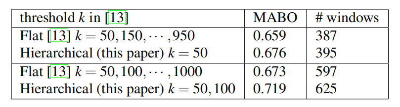
Table 2: A comparison of multiple flat partitionings against hierarchical partitionings for generating box locations shows that for the hierarchical strategy the Mean Average Best Overlap (MABO) score is consistently higher at a similar number of locations.

表2：多个平面分区与用于生成框位置的分层分区的比较表明，对于分层策略，在相同数量的位置处，平均最佳重叠（MABO）得分始终较高

As can be seen, the quality of object hypotheses is better for our hierarchical strategy than for multiple flat partitionings: At a similar number of regions, our MABO score is consistently higher. Moreover, the increase in MABO achieved by combining the locations of two variants of our hierarchical grouping algorithm is much higher than the increase achieved by adding extra thresholds for the flat partitionings. We conclude that using all locations from a hierarchical grouping algorithm is not only more natural but also more effective than using multiple flat partitionings.

可以看出，对于目标假设的质量而言，我们的分层策略比多个平面分区要好：在相同数量的区域，我们的MABO得分始终较高。此外，通过组合分层分组算法中两个变体的位置所实现的MABO的增加远远高于通过为平面分区添加额外阈值所实现的增加。我们的结论是，与使用多个平面分区相比，使用分层分组算法中的所有位置不仅更自然，而且更有效

独立的多样化策略

In this paper we propose three diversification strategies to obtain good quality object hypotheses: varying the colour space, varying the similarity measures, and varying the thresholds to obtain the starting regions. This section investigates the influence of each strategy. As basic settings we use the RGB colour space, the combination of all four similarity measures, and threshold k = 50. Each time we vary a single parameter. Results are given in Table 3.

在本文中，我们提出了三种多元化策略来获得高质量的目标假设：改变颜色空间，改变相似度，并改变阈值以获得起始区域。这一部分考察了每种策略的影响。作为基本设置，我们使用RGB颜色空间，四种相似性度量的组合，阈值k=50。每次我们改变一个参数。结果见表3。

We start examining the combination of similarity measures on the left part of Table 3. Looking first at colour, texture, size, and fill individually, we see that the texture similarity performs worst with a MABO of 0.581, while the other measures range between 0.63 and 0.64. To test if the relatively low score of texture is due to our choice of feature, we also tried to represent texture by Local Binary Patterns [24]. We experimented with 4 and 8 neighbours on different scales using different uniformity/consistency of the patterns (see [24]), where we concatenate LBP histograms of the individual colour channels. However, we obtained similar results (MABO of 0.577). We believe that one reason of the weakness of texture is because of object boundaries: When two segments are separated by an object boundary, both sides of this boundary will yield similar edge-responses, which inadvertently increases similarity.

我们开始检查表3左边的相似性度量的组合。首先分别观察颜色、纹理、大小和填充，我们发现纹理相似性在MABO为0.581时表现最差，而其他度量在0.63到0.64之间。为了测试纹理得分是否较低是因为我们选择了特征，我们还尝试用局部二值模式来表示纹理[24]。我们使用不同均匀性/一致性的图案（见[24]）在不同尺度上对4个和8个邻域进行了实验，在这些邻域中我们连接了各个颜色通道的LBP直方图。然而，我们得到了类似的结果（MABO为0.577）。我们认为，纹理弱的一个原因是由于对象边界：当两个分割被一个对象边界分开时，该边界的两边将产生相似的边缘响应，这在不经意间增加了相似性

While the texture similarity yields relatively few object locations, at 300 locations the other similarity measures still yield a MABO higher than 0.628. This suggests that when comparing individual strategies the final MABO scores in table 3 are good indicators of trade-off between quality and quantity of the object hypotheses. Another observation is that combinations of similarity measures generally outperform the single measures. In fact, using all four similarity measures perform best yielding a MABO of 0.676.

虽然纹理相似性产生的对象位置相对较少，但在300个位置，其他相似性度量仍然产生高于0.628的MABO。这表明，在比较个体策略时，表3中的最终MABO得分是衡量目标假设的质量和数量的良好指标。另一个观察结果是，相似性度量的组合通常优于单一度量。事实上，使用所有四个相似性度量可以获得0.676的MABO

Looking at variations in the colour space in the top-right of Table 3, we observe large differences in results, ranging from a MABO of 0.615 with 125 locations for the C colour space to a MABO of 0.693 with 463 locations for the HSV colour space. We note that Lab-space has a particularly good MABO score of 0.690 using only 328 boxes. Furthermore, the order of each hierarchy is effective: using the first 328 boxes of HSV colour space yields 0.690 MABO, while using the first 100 boxes yields 0.647 MABO. This shows that when comparing single strategies we can use only the MABO scores to represent the trade-off between quality and quantity of the object hypotheses set. We will use this in the next section when finding good combinations.

观察表3右上角颜色空间的变化，我们观察到结果上的巨大差异，从C颜色空间125个位置的MABO为0.615到HSV颜色空间463个位置的MABO为0.693。我们注意到Lab空间只有328个框，MABO得分为0.690。此外，每个层次的顺序是有效的：使用前328个框的HSV颜色空间产生0.690 MABO，而使用前100框能够产生0.647 MABO。这表明，在比较单一策略时，我们只能使用MABO分数来表示对象假设集的质量和数量之间的权衡。在下一节中，我们将在找到好的组合时使用这个

Experiments on the thresholds of [13] to generate the starting regions show, in the bottom-right of Table 3, that a lower initial threshold results in a higher MABO using more object locations.

在表3的右下角，对生成起始区域的阈值[13]的实验表明，较低的初始阈值导致使用更多对象位置的较高MABO

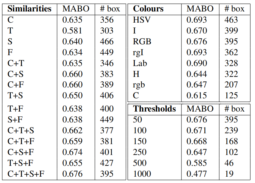
Table 3: Mean Average Best Overlap for box-based object hypotheses using a variety of segmentation strategies. (C)olour, (S)ize, and (F)ill perform similar. (T)exture by itself is weak. The best combination is as many diverse sources as possible.

表3：使用各种分割策略的基于框的对象假设的平均最佳重叠。(C)颜色，(S)大小，和(F)填充表现相似。(T)纹理本身是弱的。最好的组合是尽可能多的不同来源

多样化策略的组合

We combine object location hypotheses using a variety of complementary grouping strategies in order to get a good quality set of object locations. As a full search for the best combination is computationally expensive, we perform a greedy search using the MABO score only as optimization criterion. We have earlier observed that this score is representative for the trade-off between the number of locations and their quality.

为了得到高质量的目标定位集合，我们使用多种互补的分组策略来组合目标定位假设。由于对最佳组合的完全搜索在计算上是昂贵的，因此我们仅使用MABO得分作为优化准则来执行贪婪搜索。我们早些时候观察到，这个分数代表了定位数量和质量之间的权衡

From the resulting ordering we create three configurations: a single best strategy, a fast selective search, and a quality selective search using all combinations of individual components, i.e. colour space, similarities, thresholds, as detailed in Table 4. The greedy search emphasizes variation in the combination of similarity measures. This confirms our diversification hypothesis: In the quality version, next to the combination of all similarities, Fill and Size are taken separately. The remainder of this paper uses the three strategies in Table 4.

根据得到结果排序，我们创建了三种配置：单一最佳策略、快速选择性搜索以及在单个组件上执行所有组合（即颜色空间、相似性、阈值）的高质量选择性搜索，如表4所示。贪婪搜索强调相似性度量组合的变化。这证实了我们的多样化假设：在高质量版本中，在所有相似性的组合旁边，填充和大小是分开的。本文的其余部分使用表4中的三种策略

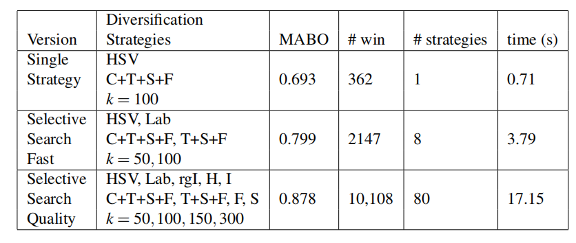
Table 4: Our selective search methods resulting from a greedy search. We take all combinations of the individual diversification strategies selected, resulting in 1, 8, and 80 variants of our hierarchical grouping algorithm. The Mean Average Best Overlap (MABO) score keeps steadily rising as the number of windows increase.

表4：贪婪搜索产生的选择性搜索方法。我们采用所选择的各个多样化策略的所有组合，得到我们的分层分组算法的1、8和80个变体。均值平均最佳重叠（MABO）分数随着窗口数的增加而稳步上升

定位质量

In this section we evaluate our selective search algorithms in terms of both Average Best Overlap and the number of locations on the Pascal VOC 2007 TEST set. We first evaluate box-based locations and afterwards briefly evaluate region-based locations.

在本节中，我们将根据平均最佳重叠和Pascal VOC 2007测试集上的定位数来评估我们的选择性搜索算法。我们首先评估基于框的定位，然后简单评估基于区域的定位

基于框的定位

We compare with the sliding window search of [16], the sliding window search of [12] using the window ratio’s of their models, the jumping windows of [34], the "objectness" boxes of [2], the boxes around the hierarchical segmentation algorithm of [3], the boxes around the regions of [9], and the boxes around the regions of [4]. From these algorithms, only [3] is not designed for finding object locations. Yet [3] is one of the best contour detectors publicly available, and results in a natural hierarchy of regions. We include it in our evaluation to see if this algorithm designed for segmentation also performs well on finding good object locations. Furthermore, [4, 9] are designed to find good object regions rather then boxes. Results are shown in Table 5 and Figure 4.

与文献[16]的滑动窗口搜索、文献[12]的滑动窗口搜索、文献[34]的跳跃窗口、文献[2]的“对象”框、文献[3]的层次分割算法框、文献[9]的区域框和文献[4]的区域框进行了比较。从这些算法中，只有[3]不是为寻找目标位置而设计的。然而[3]是公开可用的最好的轮廓检测器之一，能够得到区域的自然层次结构。我们将其包含在我们的评估中，看看这个为分割而设计的算法是否也能很好地找到好的目标位置。此外，[4，9]的设计是为了找到好的对象区域，而不是框。结果如表5和图4所示

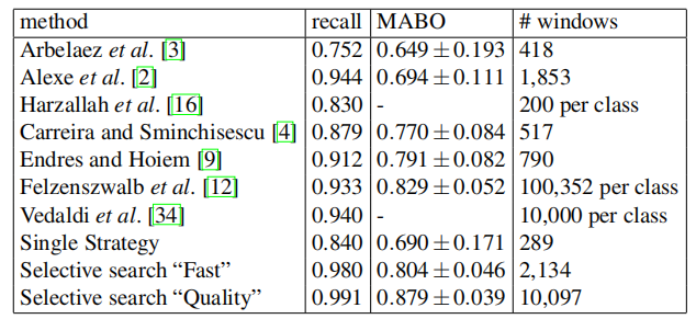
Table 5: Comparison of recall, Mean Average Best Overlap (MABO) and number of window locations for a variety of methods on the Pascal 2007 TEST set.

表5：Pascal 2007测试集上各种方法的召回率、均值平均最佳重叠（MABO）和窗口位置数的比较

Figure 4: Trade-off between quality and quantity of the object hypotheses in terms of bounding boxes on the Pascal 2007 TEST set. The dashed lines are for those methods whose quantity is expressed is the number of boxes per class. In terms of recall "Fast" selective search has the best trade-off. In terms of Mean Average Best Overlap the "Quality" selective search is comparable with [4, 9] yet is much faster to compute and goes on longer resulting in a higher final MABO of 0.879.

图4：根据Pascal 2007测试集上的边界框，在对象假设的质量和数量之间进行权衡。虚线用于那些其数量表示为每个类的框数的方法。在召回方面，"快速"选择性搜索有最好的权衡。就平均最佳重叠而言，"质量"选择搜索与[4，9]相当，但计算速度更快，持续时间更长，最终MABO更高，为0.879

As shown in Table 5, our "Fast" and "Quality" selective search methods yield a close to optimal recall of 98% and 99% respectively. In terms of MABO, we achieve 0.804 and 0.879 respectively. To appreciate what a Best Overlap of 0.879 means, Figure 5 shows for bike, cow, and person an example location which has an overlap score between 0.874 and 0.884. This illustrates that our selective search yields high quality object locations.

如表5所示，我们的"快速"和"高质量"的选择性搜索方法分别产生了98%和99%的接近最优召回率。在MABO方面，我们分别达到了0.804和0.879。为了理解0.879的最佳重叠意味着什么，图5为自行车、奶牛和人显示了一个重叠得分介于0.874和0.884之间的示例位置。这说明我们的选择性搜索可以产生高质量的对象位置

Figure 5: Examples of locations for objects whose Best Overlap score is around our Mean Average Best Overlap of 0.879. The green boxes are the ground truth. The red boxes are created using the "Quality" selective search.

图5：目标的定位示例，其最佳重叠分数约为我们的平均最佳重叠的0.879。绿色的框是正确标注。红色框是使用"质量"选择性搜索创建的

Furthermore, note that the standard deviation of our MABO scores is relatively low: 0.046 for the fast selective search, and 0.039 for the quality selective search. This shows that selective search is robust to difference in object properties, and also to image condition often related with specific objects (one example is indoor/outdoor lighting).

此外请注意，我们的MABO分数的标准差相对较低：快速选择性搜索为0.046，质量选择性搜索为0.039。这表明选择性搜索对对象特性的差异以及通常与特定对象相关的图像条件（例如室内/室外照明）具有鲁棒性

If we compare with other algorithms, the second highest recall is at 0.940 and is achieved by the jumping windows [34] using 10,000 boxes per class. As we do not have the exact boxes, we were unable to obtain the MABO score. This is followed by the exhaustive search of [12] which achieves a recall of 0.933 and a MABO of 0.829 at 100,352 boxes per class (this number is the average over all classes). This is significantly lower then our method while using at least a factor of 10 more object locations.

如果我们与其他算法相比，第二高的召回率是0.940，并且是通过跳跃窗口[34]来实现的，每个类使用10000个框。由于我们没有确切的框，我们无法获得MABO分数。接下来是对[12]的详尽搜索，在每个类100352个框（这个数字是所有类的平均值）时，召回率为0.933，MABO为0.829。这明显低于我们的方法，尽管使用了至少10倍以上的对象定位因子

Note furthermore that the segmentation methods of [4, 9] have a relatively high standard deviation. This illustrates that a single strategy can not work equally well for all classes. Instead, using multiple complementary strategies leads to more stable and reliable results.

此外，注意[4，9]的分割方法具有相对较高的标准差。这说明一个策略不能对所有类都同样有效。相反，使用多种互补策略可以获得更稳定可靠的结果

If we compare the segmentation of Arbelaez [3] with a the single best strategy of our method, they achieve a recall of 0.752 and a MABO of 0.649 at 418 boxes, while we achieve 0.875 recall and 0.698 MABO using 286 boxes. This suggests that a good segmentation algorithm does not automatically result in good object locations in terms of bounding boxes.

如果我们将Arbelaez[3]的分割与我们方法的单一最佳策略进行比较，它们在418个框中实现了0.752的召回率和0.649的MABO，而我们在286个框中实现了0.875的召回率和0.698的MABO。这表明，一个好的分割算法并不能自动地在边界框方面产生好的对象位置

Figure 4 explores the trade-off between the quality and quantity of the object hypotheses. In terms of recall, our "Fast" method outperforms all other methods. The method of [16] seems competitive for the 200 locations they use, but in their method the number of boxes is per class while for our method the same boxes are used for all classes. In terms of MABO, both the object hypotheses generation method of [4] and [9] have a good quantity/quality trade-off for the up to 790 object-box locations per image they generate. However, these algorithms are computationally 114 and 59 times more expensive than our "Fast" method.

图4探讨了目标假设的质量和数量之间的权衡。在召回方面，我们的“快速”方法优于所有其他方法。[16]的方法对于他们使用的200个位置来说似乎很有竞争力，但是在他们的方法中，框的数量是每个类的，而对于我们的方法，框作用于所有类。就MABO而言，[4]和[9]的目标假设生成方法对于生成的每幅图像多达790个对象框位置，都具有良好的数量/质量权衡。然而，这些算法的计算成本是我们的“快速”方法的114倍和59倍

Interestingly, the "objectness" method of [2] performs quite well in terms of recall, but much worse in terms of MABO. This is most likely caused by their non-maximum suppression, which suppresses windows which have more than an 0.5 overlap score with an existing, higher ranked window. And while this significantly improved results when a 0.5 overlap score is the definition of finding an object, for the general problem of finding the highest quality locations this strategy is less effective and can even be harmful by eliminating better locations.

有趣的是，[2]的“目标”方法在召回方面表现得很好，但在MABO方面表现得更差。这最有可能是由它们的非最大抑制引起的，这抑制了具有超过0.5的重叠分数的窗口以及现有的、更高等级的窗口。尽管当0.5的重叠分数是寻找目标的定义时，这显著地改善了结果，但是对于寻找最高质量位置的通用问题，这一策略效率较低，甚至通过消除更好的位置而有害

Figure 6 shows for several methods the Average Best Overlap per class. It is derived that the exhaustive search of [12] which uses 10 times more locations which are class specific, performs similar to our method for the classes bike, table, chair, and sofa, for the other classes our method yields the best score. In general, the classes with the highest scores are cat, dog, horse, and sofa, which are easy largely because the instances in the dataset tend to be big. The classes with the lowest scores are bottle, person, and plant, which are difficult because instances tend to be small. Nevertheless, cow, sheep, and tv are not bigger than person and yet can be found quite well by our algorithm.

图6显示了几个方法中每个类的平均最佳重叠。结果表明，对[12]的穷举搜索使用了10倍以上的特定于类的位置，其性能与我们对自行车、桌子、椅子和沙发类的方法相似，对于其他类，我们的方法产生最佳分数。通常，得分最高的类是cat、dog、horse和sofa，因为数据集中的实例往往很大。得分最低的班级是瓶类、人类和植物类，这类很难识别因为实例集往往很小。然而，牛、羊和电视都不比人大，而且我们的算法也能很好地找到它们

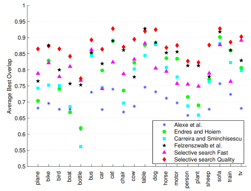
Figure 6: The Average Best Overlap scores per class for several method for generating box-based object locations on Pascal VOC 2007 TEST. For all classes but table our “Quality” selective search yields the best locations. For 12 out of 20 classes our “Fast” selective search outperforms the expensive [4, 9]. We always outperform [2].

图6：Pascal VOC 2007测试中生成基于框的目标位置的几种方法的逐类平均最佳重叠分数。对于除了表以外的所有类，我们的“质量”选择性搜索会产生最佳位置。对于20个类中的12个，我们的“快速”选择性搜索优于昂贵的[4，9]。我们总是胜过[2]

To summarize, selective search is very effective in finding a high quality set of object hypotheses using a limited number of boxes, where the quality is reasonable consistent over the object classes. The methods of [4] and [9] have a similar quality/quantity trade-off for up to 790 object locations. However, they have more variation over the object classes. Furthermore, they are at least 59 and 13 times more expensive to compute for our “Fast” and “Quality” selective search methods respectively, which is a problem for current dataset sizes for object recognition. In general, we conclude that selective search yields the best quality locations at 0.879 MABO while using a reasonable number of 10,097 class-independent object locations.

总而言之，选择性搜索在使用有限数量的框来寻找高质量的目标假设集方面非常有效，其中搜索质量在所有目标类别上是合理一致的。[4]和[9]的方法对于多达790个目标位置具有类似的质量/数量权衡。但是，它们在对象类上有更多的变化。此外，对于我们的“快速”和“质量”选择性搜索方法来说，它们的计算成本分别高出59倍和13倍，这是当前目标识别数据集大小的一个问题。一般来说，我们的结论是，选择搜索在0.879 MABO处产生最佳质量的位置，同时使用10097个类无关的对象位置的合理数目

基于区域的定位

In this section we examine how well the regions that our selective search generates captures object locations. We do this on the segmentation part of the Pascal VOC 2007 TEST set. We compare with the segmentation of [3] and with the object hypothesis regions of both [4, 9]. Table 6 shows the results. Note that the number of regions is larger than the number of boxes as there are almost no exact duplicates.

在本节中，我们将检查选择性搜索生成的区域捕获对象位置的效果。我们在Pascal VOC 2007测试集的分割部分执行此操作。我们比较了[3]的分割和[4，9]的目标假设区域。结果如表6所示。请注意，区域数大于框数，因为几乎没有完全重复的区域

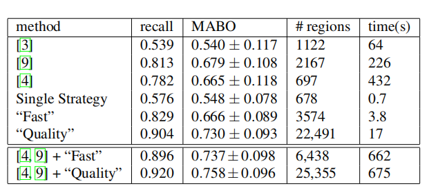
Table 6: Comparison of algorithms to find a good set of potential object locations in terms of regions on the segmentation part of Pascal 2007 TEST.

表6：根据Pascal 2007测试的分割部分，比较能够找到一组好的潜在目标位置的算法

The object regions of both [4, 9] are of similar quality as our “Fast” selective search, 0.665 MABO and 0.679 MABO respectively where our “Fast” search yields 0.666 MABO. While [4, 9] use fewer regions these algorithms are respectively 114 and 59 times computationally more expensive. Our “Quality” selective search generates 22,491 regions and is respectively 25 and 13 times faster than [4, 9], and has by far the highest score of 0.730 MABO.

文章[4，9]的目标区域质量与我们的“快速”选择性搜索相似，分别为0.665和0.679 MABO，其中我们的“快速”搜索产生0.666 MABO。虽然[4，9]使用较少的区域，但这些算法的计算成本分别是前者的114倍和59倍。我们的“质量”选择性搜索产生22491个区域，分别比[4,9]快25和13倍，目前最高得分为0.730 MABO

Figure 7 shows the Average Best Overlap of the regions per class. For all classes except bike, our selective search consistently has relatively high ABO scores. The performance for bike is disproportionally lower for region-locations instead of object-locations, because bike is a wire-frame object and hence very difficult to accurately delineate.

图7显示了每个类区域的平均最佳重叠。对于除自行车以外的所有类别，我们的选择性搜索始终具有相对较高的ABO分数。由于自行车是一个线框物体，因此很难准确地描绘出来，因此自行车在区域定位上的性能比目标定位上的性能低得多

Figure 7: Comparison of the Average Best Overlap Scores per class between our method and others on the Pascal 2007 TEST set. Except for train, our “Quality” method consistently yields better Average Best Overlap scores.

图7:Pascal 2007测试集上我们的方法和其他方法的平均最佳重叠分数的比较。除了火车类别之外，我们的“质量”方法始终能获得更好的平均最佳重叠分数

If we compare our method to others, the method of [9] is better for train, for the other classes our “Quality” method yields similar or better scores. For bird, boat, bus, chair, person, plant, and tv scores are 0.05 ABO better. For car we obtain 0.12 higher ABO and for bottle even 0.17 higher ABO. Looking at the variation in ABO scores in table 6, we see that selective search has a slightly lower variation than the other methods: 0.093 MABO for “quality” and 0.108 for [9]. However, this score is biased because of the wire-framed bicycle: without bicycle the difference becomes more apparent. The standard deviation for the “quality” selective search becomes 0.058, and 0.100 for [9]. Again, this shows that by relying on multiple complementary strategies instead of a single strategy yields more stable results.

如果我们将我们的方法与其他方法进行比较，[9]的方法更适合训练，对于其他类别，我们的“质量”方法可以得到相似或更好的分数。鸟、船、公共汽车、椅子、人、植物和电视的得分比其他算法高出0.05 ABO。对于汽车，我们高出0.12 ABO，对于瓶子，甚至高出0.17 大小ABO。通过观察表6中ABO得分的方差，我们发现选择性搜索的方差比其他方法略低：“质量”选择性搜索有0.093 MABO，文章[9]有0.108。然而因为铁丝线框自行车的影响，这个分数是有偏差的：除去自行车后差异会变得更加明显。“质量”选择性搜索的标准差变为0.058，而[9]的标准差变为0.100。这再次表明依靠多种互补策略而不是单一策略可以产生更稳定的结果

Figure 8 shows several example segmentations from our method and [4, 9]. In the first image, the other methods have problems keeping the white label of the bottle and the book apart. In our case, one of our strategies ignores colour while the “fill” similarity (Eq. 5) helps grouping the bottle and label together. The missing bottle part, which is dusty, is already merged with the table before this bottle segment is formed, hence “fill” will not help here. The second image is an example of a dark image on which our algorithm has generally strong results due to using a variety of colour spaces. In this particular image, the partially intensity invariant Lab colour space helps to isolate the car. As we do not use the contour detection method of [3], our method sometimes generates segments with an irregular border, which is illustrated by the third image of a cat. The final image shows a very difficult example, for which only [4] provides an accurate segment.

图8显示了我们的方法和[4，9]中的几个示例分割。在第一张图片中，其他方法无法将瓶子和书本的白色标签分开。在我们的例子中，我们的策略之一是忽略颜色，而“填充”相似性（公式5）有助于将瓶子和标签组合在一起。缺少的瓶子部分充满灰尘，所以在瓶子分割组合之前已经合并到桌子，因此“填充”不起作用。第二幅图像是一幅深色图像的例子，由于使用了多种颜色空间，我们的算法通常有很强的效果。在这个特殊的图像中，部分强度不变的Lab颜色空间有助于隔离汽车。由于我们没有使用[3]中的轮廓检测方法，我们的方法有时会生成具有不规则边界的线段，如猫的第三幅图像所示。最后的图像显示了一个非常困难的例子，只有[4]提供了一个精确的分割

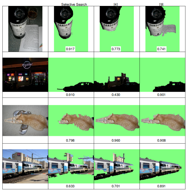
Figure 8: A qualitative comparison of selective search, [4], and [9]. For our method we observe: ignoring colour allows finding the bottle, multiple colour spaces help in dark images (car), and not using [3] sometimes result in irregular borders such as the cat.

图8：选择性搜索与[4]和[9]的定性比较。对于我们的方法，我们观察到：忽略颜色可以找到瓶子，多个颜色空间有助于深色图像（汽车），不使用[3]有时会导致不规则的边界，如猫

Now because of the nature of selective search, rather than pitting methods against each other, it is more interesting to see how they can complement each other. As both [4, 9] have a very different algorithm, the combination should prove effective according to our diversification hypothesis. Indeed, as can be seen in the lower part of Table 6, combination with our “Fast” selective search leads to 0.737 MABO at 6,438 locations. This is a higher MABO using less locations than our “quality” selective search. A combination of [4, 9] with our “quality” sampling leads to 0.758 MABO at 25,355 locations. This is a good increase at only a modest extra number of locations.

现在，因为选择性搜索的本质不是将方法相互对立，所以更有趣的是看看它们如何能够相互补充。由于[4,9]都有一个非常不同的算法，根据我们的多样化假设，这种组合应该证明是有效的。事实上，如表6的下半部分所示，结合我们的“快速”选择性搜索，在6438个位置找到0.737 MABO。这是一个比我们的“质量”选择性搜索更高的MABO，而且拥有更少的定位。结合[4，9]和我们的“质量”方法进行采样，在25355个地点得到0.758 MABO。在只有少量额外定位的情况下是一个很好的增长

To conclude, selective search is highly effective for generating object locations in terms of regions. The use of a variety of strategies makes it robust against various image conditions as well as the object class. The combination of [4], [9] and our grouping algorithms into a single selective search showed promising improvements. Given these improvements, and given that there are many more different partitioning algorithms out there to use in a selective search, it will be interesting to see how far our selective search paradigm can still go in terms of computational efficiency, number of object locations, and the quality of object locations.

综上所述，选择性搜索对于根据区域生成目标位置而言是非常有效的。多种策略的使用使得它对各种图像条件和对象类都具有鲁棒性。将[4]、[9]和我们的分组算法组合成一个单一的选择性搜索显示出有希望的改进。考虑到这些改进，以及有更多不同的分区算法可用于选择性搜索，看看我们的选择性搜索范式在计算效率、目标定位数量和质量方面还能走多远

目标识别

In this section we will evaluate our selective search strategy for object recognition using the Pascal VOC 2010 detection task.

在本节中，我们将使用Pascal VOC 2010检测任务评估用于目标识别的选择性搜索策略

Our selective search strategy enables the use of expensive and powerful image representations and machine learning techniques. In this section we use selective search inside the Bag-of-Words based object recognition framework described in Section 4. The reduced number of object locations compared to an exhaustive search make it feasible to use such a strong Bag-of-Words implementation.

我们的选择性搜索策略能够使用昂贵而强大的图像表示和机器学习技术。本节中我们在第4部分描述的基于词袋的目标识别框架中使用选择性搜索。与穷举搜索相比，目标定位数量的减少使得使用这样一个强大的词袋实现成为可能

To give an indication of computational requirements: The pixel-wise extraction of three SIFT variants plus visual word assignmenttakes around 10 seconds and is done once per image. The final round of SVM learning takes around 8 hours per class on a GPU for approximately 30,000 training examples [33] resulting from two rounds of mining negatives on Pascal VOC 2010. Mining hard negatives is done in parallel and takes around 11 hours on 10 machines for a single round, which is around 40 seconds per image. This is divided into 30 seconds for counting visual word frequencies and 0.5 seconds per class for classification. Testing takes 40 seconds for extracting features, visual word assignment, and counting visual word frequencies, after which 0.5 seconds is needed per class for classification. For comparison, the code of [12] (without cascade, just like our version) needs for testing slightly less than 4 seconds per image per class. For the 20 Pascal classes this makes our framework faster during testing.

给出计算要求的指示：三个SIFT变体的像素级提取加上视觉单词分配大约需要10秒，并且每个图像执行一次。最后一轮的SVM学习在GPU上花费大约8个小时一个类，大约30000个训练示例（33），进行两轮PASCAL VOC 2010的负样本挖掘。挖掘hard negatives是并行进行的，每一轮需要在10台机器花费大约11个小时，每张图片大约40秒。这被分为30秒用于统计可视单词频率，0.5秒用于分类。测试需要40秒来提取特征、可视化单词分配和统计可视化单词的频率，之后每个类需要0.5秒来进行分类。为了进行比较，[12]的代码（没有级联，就像我们的版本一样）需要对每个类的每个图像进行不到4秒的测试。对于20个Pascal类而言，我们的框架在测试期间更快

We evaluate results using the official evaluation server. This evaluation is independent as the test data has not been released. We compare with the top-4 of the competition. Note that while all methods in the top-4 are based on an exhaustive search using variations on part-based model of [12] with HOG-features, our method differs substantially by using selective search and Bag-of-Words features. Results are shown in Table 7.

我们使用官方评估服务器评估结果。此评估是独立的，因为测试数据尚未发布。我们和比赛的前4名进行比较。请注意，虽然排名前4位的所有方法都是基于使用具有HOG特征的[12]的基于part的模型的变体的穷举搜索，但是我们的方法通过使用选择性搜索和词袋特征而有本质的不同。结果见表7

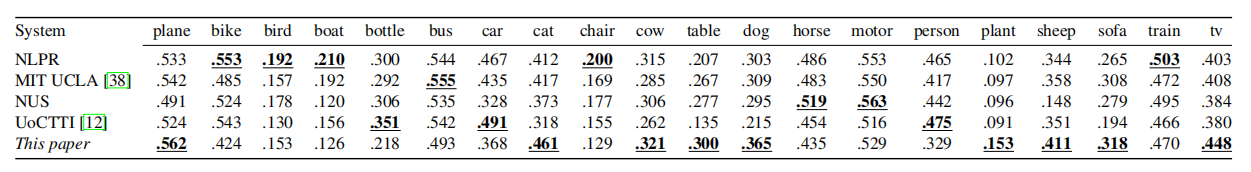
Table 7: Results from the Pascal VOC 2010 detection task test set. Our method is the only object recognition system based on Bag-of-Words. It has the best scores for 9, mostly non-rigid object categories, where the difference is up to 0.056 AP. The other methods are based on part-based HOG features, and perform better on most rigid object classes.

表7:Pascal VOC 2010检测任务测试集的结果。我们的方法是唯一一个基于词袋的目标识别系统。它有9个最好的分数，大多是非刚性物体类别，其中差异高达0.056 AP。其他方法基于基于部分的HOG特征，并且在大多数刚性目标类上执行得更好

It is shown that our method yields the best results for the classes plane, cat, cow, table, dog, plant, sheep, sofa, and tv. Except table, sofa, and tv, these classes are all non-rigid. This is expected, as Bag-of-Words is theoretically better suited for these classes than the HOG-features. Indeed, for the rigid classes bike, bottle, bus, car, person, and train the HOG-based methods perform better. The exception is the rigid class tv. This is presumably because our selective search performs well in locating tv’s, see Figure 6.

结果表明，该方法对平面类、猫类、牛类、桌子类、狗类、植物类、羊类、沙发类、电视类的学习效果最好。除了桌子、沙发和电视，这些类都是非刚性的。这是意料之中的，因为理论上，词袋比HOG特性更适合这些类。事实上，对于刚性类，比如自行车、瓶子、公共汽车、汽车、人和火车，基于HOG的方法表现得更好。除了tv是个意外。这可能是因为我们的选择性搜索在电视定位上表现良好，见图6

In the Pascal 2011 challenge there are several entries wich achieve significantly higher scores than our entry. These methods use Bag-of-Words as additional information on the locations found by their part-based model, yielding better detection accuracy. Interestingly, however, by using Bag-of-Words to detect locations our method achieves a higher total recall for many classes [10].

在2011年Pascal挑战赛中，有几个参赛者的得分明显高于我们的参赛者。这些方法使用词袋作为基于部分模型发现的定位i的附加信息，从而获得更好的检测精度。然而，有趣的是，通过使用词袋来检测定位，我们的方法对许多类实现了更高的总召回率[10]

Finally, our selective search enabled participation to the detection task of the ImageNet Large Scale Visual Recognition Challenge 2011 (ILSVRC2011) as shown in Table 8. This dataset contains 1,229,413 training images and 100,000 test images with 1,000 different object categories. Testing can be accelerated as features extracted from the locations of selective search can be reused for all classes. For example, using the fast Bag-of-Words framework of [30], the time to extract SIFT-descriptors plus two colour variants takes 6.7 seconds and assignment to visual words takes 1.7 seconds. Using a 1x1, 2x2, and 3x3 spatial pyramid division it takes 14 seconds to get all 172,032 dimensional features. Classification in a cascade on the pyramid levels then takes 0.3 seconds per class. For 1,000 classes, the total process then takes 323 seconds per image for testing. In contrast, using the part-based framework of [12] it takes 3.9 seconds per class per image, resulting in 3900 seconds per image for testing. This clearly shows that the reduced number of locations helps scaling towards more classes.

最后，我们的选择性搜索使我们能够参与ImageNet大规模视觉识别挑战2011（ILSVRC2011）的检测任务，如表8所示。该数据集包含1229413个训练图像和100000个具有1000个不同对象类别的测试图像。测试可以加速，因为从选择性搜索位置提取的特征可以对所有类重用。例如，使用[30]的快速词袋框架，提取SIFT描述符和两个颜色变体所需的时间为6.7秒，而指定给可视化单词所需的时间为1.7秒。使用1x1、2x2和3x3空间金字塔分割，需要14秒才能获得所有172032维特征。在金字塔级别上进行级联分类，每个类需要0.3秒。对于1000个类，测试每张图片的过程需要323秒。相反，使用[12]中基于部件的框架，每个类的每个图像需要3.9秒，因此测试完所有图像需要3900秒。这清楚地表明，减少的位置数量有助于向更多类扩展

We conclude that compared to an exhaustive search, selective search enables the use of more expensive features and classifiers and scales better as the number of classes increase.

我们的结论是，与穷举搜索相比，选择性搜索能够使用更昂贵的特征和分类器，并且随着类数的增加，搜索的规模会更好

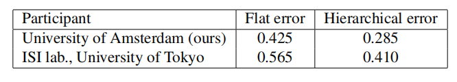
Table 8: Results for ImageNet Large Scale Visual Recognition Challenge 2011 (ILSVRC2011). Hierarchical error penalises mistakes less if the predicted class is semantically similar to the real class according to the WordNet hierarchy.

表8:ImageNet 2011年大规模视觉识别挑战赛（ILSVRC2011）结果。根据WordNet的层次结构，如果预测的类在语义上与实际类相似，那么层次错误对错误的惩罚较小

Pascal VOC 2012

Because the Pacal VOC 2012 is the latest and perhaps final VOC dataset, we briefly present results on this dataset to facilitate comparison with our work in the future. We present quality of boxes using the TRAIN+VAL set, the quality of segments on the segmentation part of TRAIN+VAL, and our localisation framework using a Spatial Pyramid of 1x1, 2x2, 3x3, and 4x4 on the TEST set using the official evaluation server.

因为Pacal VOC 2012是最新的，也许是最终的VOC数据集，我们简要介绍了这个数据集的结果，以便于与我们未来的工作进行比较。我们使用TRAIN+VAL集呈现框的质量，在TRAIN+VAL的分割部分呈现分割质量，以及使用官方评估服务器在测试集上使用1x1、2x2、3x3和4x4的空间金字塔的定位框架

Results for the location quality are presented in table 9. We see that for the box-locations the results are slightly higher than in Pascal VOC 2007. For the segments, however, results are worse. This is mainly because the 2012 segmentation set is considerably more difficult.

定位质量结果见表9。我们看到，对于框定位，结果略高于Pascal VOC 2007。然而，对于分割而言，结果更糟。这主要是因为2012年的分割设置要困难得多

For the 2012 detection challenge, the Mean Average Precision is 0.350. This is similar to the 0.351 MAP obtained on Pascal VOC 2010.

对于2012年的检测挑战，均值平均精度为0.350。这与Pascal VOC 2010上获得的0.351 MAP相似

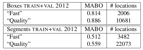
Table 9: Quality of locations on Pascal VOC 2012 TRAIN+VAL.

表9:Pascal VOC 2012 TRAIN+VAL上的定位质量

定位质量的上限

In this experiment we investigate how close our selective search locations are to the optimal locations in terms of recognition accuracy for Bag-of-Words features. We do this on the Pascal VOC 2007 TEST set.

在这个实验中，我们研究了我们的选择性搜索定位与最佳定位的接近程度，以确定词袋特征的识别精度。我们在PASCAL VOC 2007测试集上完成

The red line in Figure 9 shows the MAP score of our object recognition system when the top n boxes of our “quality” selective search method are used. The performance starts at 0.283 MAP using the first 500 object locations with a MABO of 0.758. It rapidly increases to 0.356 MAP using the first 3000 object locations with a MABO of 0.855, and then ends at 0.360 MAP using all 10,097 object locations with a MABO of 0.883.

图9中的红线显示了使用“质量”选择性搜索方法得到的前n个框时，我们的目标识别系统的MAP成绩。使用MABO为0.758的前500个对象位置能够得到0.293 MAP的性能。使用前3000个目标定位（MABO为0.855）能够快速增加到0.356 MAP，最后使用所有10097个目标位置（MABO为0.883）能够得到0.360 MAP

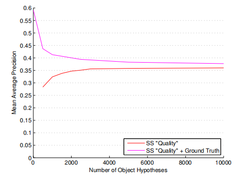
Figure 9: Theoretical upper limit for the box selection within our object recognition framework. The red curve denotes the performance using the top n locations of our “quality” selective search method, which has a MABO of 0.758 at 500 locations, 0.855 at 3000 locations, and 0.883 at 10,000 locations. The magenta curve denotes the performance using the same top n locations but now combined with the ground truth, which is the upper limit of location quality (MABO = 1). At 10,000 locations, our object hypothesis set is close to optimal in terms of object recognition accuracy.

图9：目标识别框架中选择框的理论上限。红色曲线表示使用我们的“质量”选择性搜索方法的前n个位置的性能，该方法在500个位置的MABO为0.758，在3000个位置的MABO为0.855，在10000个位置的MABO为0.883。洋红色曲线表示使用相同的前n个位置的性能，同时结合了ground truth，这是定位质量的上限（MABO=1）。在10000个位置，我们的目标假设集在目标识别精度方面接近最优

The magenta line shows the performance of our object recognition system if we include the ground truth object locations to our hypotheses set, representing an object hypothesis set of “perfect” quality with a MABO score of 1. When only the ground truth boxes are used a MAP of 0.592 is achieved, which is an upper bound of our object recognition system. However, this score rapidly declines to 0.437 MAP using as few as 500 locations per image. Remarkably, when all 10,079 boxes are used the performance drops to 0.377 MAP, only 0.017 MAP more than when not including the ground truth. This shows that at 10,000 object locations our hypotheses set is close to what can be optimally achieved for our recognition framework. The most likely explanation is our use of SIFT, which is designed to be shift invariant [21]. This causes approximate boxes, of a quality visualised in Figure 5, to be still good enough. However, the small gap between the “perfect” object hypotheses set of 10,000 boxes and ours suggests that we arrived at the point where the degree of invariance for Bag-of-Words may have an adverse effect rather than an advantageous one.

如果我们在假设集中包含了ground truth目标定位，那么洋红线表明了我们的目标识别系统的性能，表示了一个具有“完美”质量（MABO分数为1）目标假设集。当只使用ground truth框时，可以得到0.592 MAP，这是我们的目标识别系统的上限。然而，当每张图像仅有500个定位时，这一得分迅速下降到0.437 MAP。值得注意的是，当使用所有10079个盒子时，性能下降到0.377 MAP，仅比不包括ground truth多0.017 MAP。这表明，拥有10000个目标定位时，我们的假设集接近于我们的识别框架所能达到的最佳效果。最有可能的解释是我们使用了SIFT，它被设计为移位不变量[21]。这就导致了图5所示质量近似框仍然足够好。然而，10000个框的“完美”目标假设集和我们的假设集之间的小差距表明，我们到达了这样一个点：对词袋的不变性程度可能产生不利影响，而不是有利影响

The decrease of the “perfect” hypothesis set as the number of boxes becomes larger is due to the increased difficulty of the problem: more boxes means a higher variability, which makes the object recognition problem harder. Earlier we hypothesized that an exhaustive search examines all possible locations in the image, which makes the object recognition problem hard. To test if selective search alleviates the problem, we also applied our Bag-of-Words object recognition system on an exhaustive search, using the locations of [12]. This results in a MAP of 0.336, while the MABO was 0.829 and the number of object locations 100,000 per class. The same MABO is obtained using 2,000 locations with selective search. At 2,000 locations, the object recognition accuracy is 0.347. This shows that selective search indeed makes the problem easier compared to exhaustive search by reducing the possible variation in locations.

随着框数量的增加，“完美”假设集的减少是由于问题难度的增加：盒子越多意味着可变性越高，这使得目标识别问题更加困难。之前我们假设一个详尽的搜索检查能够得到图像中所有可能位置，这使得目标识别问题变得困难。为了测试选择性搜索是否缓解了这个问题，我们还使用了我们的词袋目标识别系统，使用了[12]中的位置进行穷举搜索。这将得到0.336 MAP，而MABO为0.829，每个类的目标定位数为100000。使用2000个定位的选择性搜索可以得到相同的MABO。在2000个定位中目标识别精度为0.347。这表明，通过减少定位的可能，选择性搜索确实比穷举搜索更容易解决问题

To conclude, there is a trade-off between quality and quantity of object hypothesis and the object recognition accuracy. High quality object locations are necessary to recognise an object in the first place. Being able to sample fewer object hypotheses without sacrificing quality makes the classification problem easier and helps to improves results. Remarkably, at a reasonable 10,000 locations, our object hypothesis set is close to optimal for our Bag-of-Words recognition system. This suggests that our locations are of such quality that features with higher discriminative power than is normally found in Bag-of-Words are now required.

总之，目标假设的质量与目标识别的准确性之间存在着一种权衡关系。高质量的物体定位是识别物体所必需的。能够在不牺牲质量的情况下对较少的目标假设进行采样，使得分类问题变得更容易，并有助于改进结果。值得注意的是，在10000个定位上，我们的目标假设集接近于我们的词袋识别系统的最优值。这表明我们的定位特征拥有比通常在词袋中发现的具有更高辨别力

总结

This paper proposed to adapt segmentation for selective search. We observed that an image is inherently hierarchical and that there are a large variety of reasons for a region to form an object. Therefore a single bottom-up grouping algorithm can never capture all possible object locations. To solve this we introduced selective search, where the main insight is to use a diverse set of complementary and hierarchical grouping strategies. This makes selective search stable, robust, and independent of the object-class, where object types range from rigid (e.g. car) to non-rigid (e.g. cat), and theoretically also to amorphous (e.g. water).

本文提出了一种适用于选择性搜索的分割方法。我们观察到，图像本身是分层的，一个区域形成一个对象有很多原因。因此，单一的自底向上分组算法永远无法捕获所有可能的目标位置。为了解决这个问题，我们引入了选择性搜索，其中的主要观点是使用一组不同的互补和分层的分组策略。这使得选择性搜索稳定、健壮，并且独立于对象类，其中对象类型从刚性（例如car）到非刚性（例如cat），理论上也适用于非晶态（例如water）

In terms of object windows, results show that our algorithm is superior to the “objectness” of [2] where our fast selective search reaches a quality of 0.804 Mean Average Best Overlap at 2,134 locations. Compared to [4, 9], our algorithm has a similar trade-off between quality and quantity of generated windows with around 0.790 MABO for up to 790 locations, the maximum that they generate. Yet our algorithm is 13-59 times faster. Additionally, it creates up to 10,097 locations per image yielding a MABO as high as 0.879.

在目标窗口方面，我们的算法优于[2]，在2134个位置，我们的快速选择性搜索达到0.804的平均最佳重叠质量。与[ 4, 9 ]相比，我们的算法在生成窗口的质量和数量上有相似的权衡，最多790个位置，大约0.790 MABO。然而我们的算法快13-59倍。此外，它可以为每个图像创建多达10097个位置，产生高达0.879的MABO

In terms of object regions, a combination of our algorithm with [4, 9] yields a considerable jump in quality (MABO increases from 0.730 to 0.758), which shows that by following our diversification paradigm there is still room for improvement.

在目标区域方面，将我们的算法与[4，9]相结合，在质量上有了相当大的提升（MABO从0.730增加到0.758），这表明，遵循我们的多样化模式仍有改进的空间

Finally, we showed that selective search can be successfully used to create a good Bag-of-Words based localisation and recognition system. In fact, we showed that quality of our selective search locations are close to optimal for our version of Bag-of-Words based object recognition.

最后，我们证明了选择性搜索可以成功地用于创建一个良好的基于词袋的定位和识别系统。事实上，我们已经证明了我们的选择性搜索定位的质量对于我们的基于词袋的目标识别来说是接近最优的

大海