[GoogLeNet]Inception_v2
论文Rethinking the Inception Architecture for Computer Vision对GoogLeNet和GoogleNet_BN的实现做了进一步的解释,同时提出了新的Inception模块和损失函数LSR(label-smoothing regularizer),本文实现其中的Inception_v2架构
论文翻译地址:[译]Rethinking the Inception Architecture for Computer Vision
分解大滤波器尺寸卷积
文章提出了两种分解大尺度卷积核的方式
- 分解成更小的卷积
- 非对称卷积的空间分解
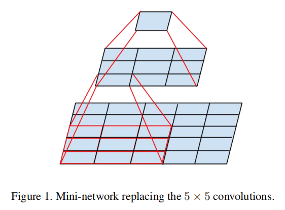
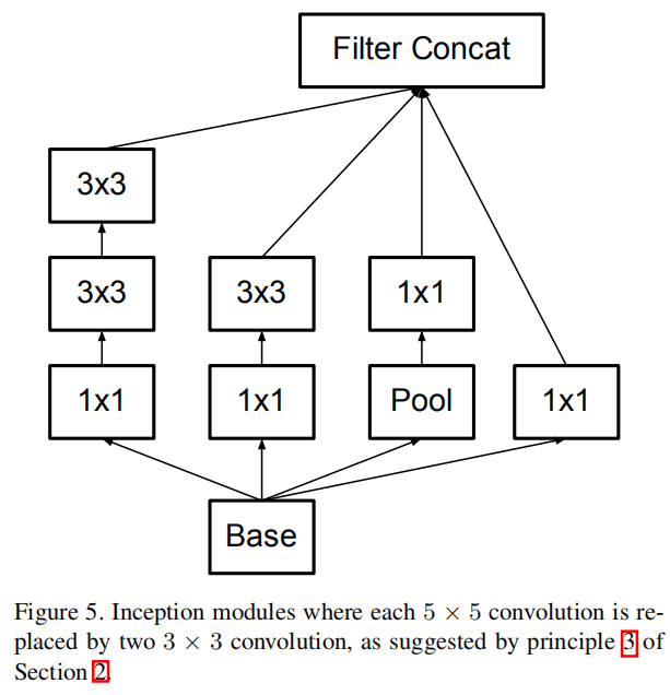
分解成更小的卷积
大尺寸卷积滤波器具有捕捉早期层中更远单元的激活之间的信号相关性的优点,不过其缺点在于高参数,计算耗时。一种分解方式是使用更小的卷积核网络来替代大卷积,这样能够有效减少参数数目,比如使用两个9/25=0.36
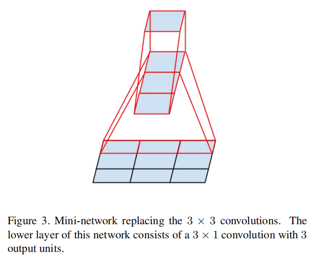
非对称卷积的空间分解
另一种方式就是使用非对称卷积来替换大尺寸卷积滤波器,比如使用
论文通过实验发现使用这种因子分解在早期层上不能很好地工作,但是它在中等网格尺寸上给出了非常好的结果(在12和20之间)。在这个水平上,通过使用
辅助分类器
在GoogLeNet模型的训练过程中,网络早期层额外使用了两个分类器,其最初的动机是将有用的梯度推至较低层,实现权重训练,通过在极深网络中对抗消失梯度问题来改善训练期间的收敛性。论文经过实验发现辅助分类器在训练的早期并没有改善收敛。但是接近训练结束时,带有辅助分支的网络开始超越没有任何辅助分支的网络的精度,并达到稍高的平台。
论文实验后发现辅助分类器起着正则化的作用;移除较低(4a)的辅助分支对网络的最终质量没有任何不利影响
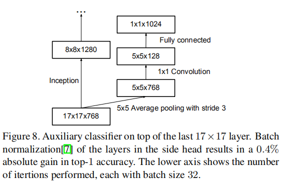
辅助分类器的实现参数也发生了变化
- 使用
大小,步长为 的平均池化,输出为 - 进行
卷积,输出为 - 全连接操作,权重大小为
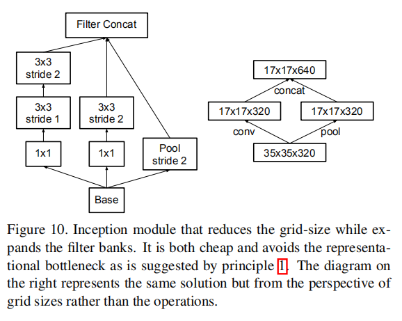
网格衰减
论文提出了一种有效衰减网络尺寸的方法,在Inception模块中通过并行计算卷积层和池化层(步长为2,实现空间尺寸减少),然后按深度维度连接在一起。这种方式比之前实现的先卷积后池化的操作更有效
Inception-v2
论文中给出了Inception-v2模块的架构:
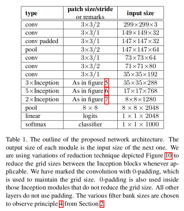
其中前3个Inception模块使用之前的实现,如下图所示:
中间5个Inception模块进行了非对称卷积分解,如下图所示:
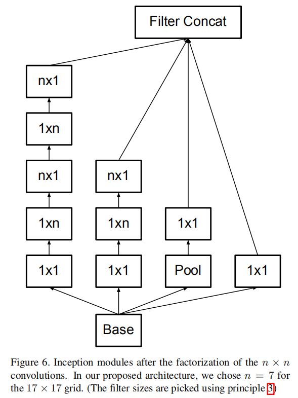
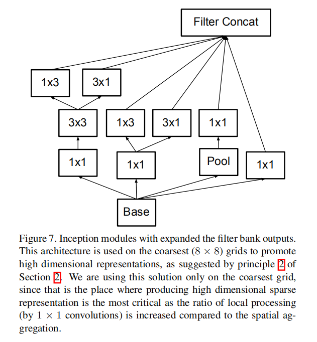
最后2个Inception模块采用了网格缩减方法,如下图所示:
参数推导
文章并没有给出完整的实现,在网上也找了很久没有找到:
The detailed structure of the network, including the sizes of filter banks inside the Inception modules, is given in the supplementary material, given in the model.txt that is in the tar-file of this submission.
自己设计了一些参数进行推导实现.假定输入大小为
- 前期卷积和池化操作
- 第一个
Inception组(前3个Inception模块) - 第二个
Inception组(中间5个Inception模块) - 第三个
Inception组(最后2个Inception模块) - 最后的卷积池化操作
前期卷积和池化操作
第一个Inception组
For the Inception part of the network, we have 3 traditional inception modules at the 35×35 with 288 filters each.
前3个Inception模块包含了288个滤波器,输入
| type | 步长 | 输出大小 | #1x1 | #3x3 reduce | #3x3 | double #3x3 reduce | double #3x3 | Pool+proj |
|---|---|---|---|---|---|---|---|---|
| inception(3a) | 35x35x288 | 64 | 64 | 64 | 64 | 96 | Avg+64 | |
| Inception(3b) | 35x35x288 | 64 | 64 | 96 | 64 | 96 | Avg+32 | |
| Inception(3c) | Stride 2 | 17x17x768 | 0 | 128 | 320 | 64 | 160 | Max+0 |
上述操作中:
- 将
卷积进一步拆分成两个 小卷积网络,这两个 卷积拥有相同大小的卷积核以及滤波器数目 - 前两层使用
,最后一层使用 ,且后续不连接 卷积
后续操作遵循上述原则
第二个Inception组
This is reduced to a 17 × 17 grid with 768 filters using the grid reduction technique described in section 5. This is is followed by 5 instances of the factorized inception modules as depicted in figure 5. This is reduced to a 8 × 8 × 1280 grid with the grid reduction technique depicted in figure 10.
中间5个Inception模块包含了768个滤波器,输入
| type | 步长 | 输出大小 | #1x1 | #7x7 reduce | #7x7 | double #7x7 reduce | double #3x3 | Pool+proj |
|---|---|---|---|---|---|---|---|---|
| Inception(5a) | 17x17x768 | 192 | 96 | 160 | 96 | 160 | Avg+256 | |
| Inception(5b) | 17x17x768 | 192 | 96 | 160 | 96 | 160 | Avg+256 | |
| Inception(5c) | 17x17x768 | 192 | 96 | 160 | 96 | 160 | Avg+256 | |
| Inception(5d) | 17x17x768 | 192 | 96 | 160 | 96 | 160 | Avg+256 | |
| Inception(5e) | Stride 2 | 8x8x1280 | 0 | 128 | 192 | 128 | 320 | Max+0 |
第三个Inception组
At the coarsest 8 × 8 level, we have two Inception modules as depicted in figure 6, with a concatenated output filter bank size of 2048 for each tile.
最后2个Inception模块包含了1280个滤波器,输入
| type | 步长 | 输出大小 | #1x1 | #3x3 reduce | #3x3 | double #3x3 reduce | double #3x3 | Pool+proj |
|---|---|---|---|---|---|---|---|---|
| Inception(2a) | 8x8x1280 | 256 | 128 | 160 | 128 | 240 | Avg+224 | |
| Inception(2b) | 8x8x2048 | 256 | 96 | 96 | 96 | 160 | Max+0 |
模块采样非对称卷积运算,并且分解
- 第一层:$256+1602+2402+224=1280$
- 第二层:$256+962+1602+1280=2048$
最后的卷积池化操作
PyTorch
参考:inception.py
关键在于实现3种不同类型的Inception模块,依次命名为:InceptionA/InceptionB/InceptionC。具体实现参考 zjZSTU/GoogLeNet
训练
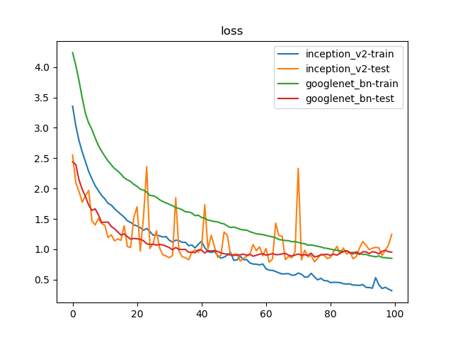
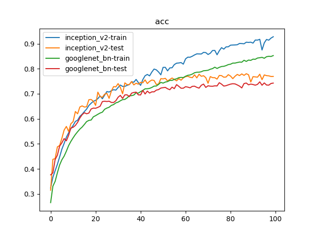
比对Inception_v2实现以及GoogLeNet_BN模型。训练参数如下:
- 数据集:
PASCAL VOC 07+12,20类共40058个训练样本和12032个测试样本 - 批量大小:
128 - 优化器:
Adam,学习率为1e-3 - 随步长衰减:每隔
8轮衰减4%,学习因子为0.96 - 迭代次数:
100轮
1 | {'train': 40058, 'test': 12032} |
100轮迭代后,Inception_v2实现了78.02%的最好测试精度;GoogLeNet_BN实现了74.77%的最好测试精度