[LR Scheduler]如何找到最优学习率
如何寻找最优学习率?
根据准确度寻找最优学习率
论文Cyclical Learning Rates for Training Neural Networks提出了周期学习率调度方法,让学习率在合理的边界值之间循环变化(不再单调递减)
摘要
It is known that the learning rate is the most important hyper-parameter to tune for training deep neural networks. This paper describes a new method for setting the learning rate, named cyclical learning rates, which practically eliminates the need to experimentally find the best values and schedule for the global learning rates. Instead of monotonically decreasing the learning rate, this method lets the learning rate cyclically vary between reasonable boundary values. Training with cyclical learning rates instead of fixed values achieves improved classification accuracy without a need to tune and often in fewer iterations. This paper also describes a simple way to estimate “reasonable bounds” – linearly increasing the learning rate of the network for a few epochs. In addition, cyclical learning rates are demonstrated on the CIFAR-10 and CIFAR-100 datasets with ResNets, Stochastic Depth networks, and DenseNets, and the ImageNet dataset with the AlexNet and GoogLeNet architectures. These are practical tools for everyone who trains neural networks.
众所周知,学习率是用于训练深层神经网络最重要的超参数。本文描述了一种设置学习率的新方法,称为循环学习率,它实际上消除了通过实验找到全局学习率的最佳值和调度方法的需要。该方法不再单调降低学习率,而是让学习率在合理的边界值之间循环变化。用循环学习率而不是固定值进行训练,可以提高分类精度,而不需要调整,而且迭代次数更少。本文还描述了一种估计“合理边界”的简单方法 - 在几个周期内线性增加网络的学习率。此外,在CIFAR-10和CIFAR-100数据集上使用ResNets、随机深度网络和DenseNet测试了循环学习率,并且在ImageNet数据集上使用AlexNet和GoogLeNet架构进行测试。实践证明循环学习率是训练神经网络的实用工具
3.3. How can one estimate reasonable minimum and maximum boundary values?
There is a simple way to estimate reasonable minimum and maximum boundary values with one training run of the network for a few epochs. It is a “LR range test”; run your model for several epochs while letting the learning rate increase linearly between low and high LR values. This test is enormously valuable whenever you are facing a new architecture or dataset.
有一种简单的方法可以估计合理的最小和最大边界值,只需在几个周期内对网络进行训练即可。这是一个LR range test;运行几个周期,让学习率从低到高线性增加。每当你面对一个新的架构或数据集时,这个测试都是非常有价值的
The triangular learning rate policy provides a simple mechanism to do this. For example, in Caffe, set
base_lrto the minimum value and setmax_lrto the maximum value. Set both theand max_iterto the same number of iterations. In this case, the learning rate will increase linearly from the minimum value to the maximum value during this short run. Next, plot the accuracy versus learning rate. Note the learning rate value when the accuracy starts to increase and when the accuracy slows, becomes ragged, or starts to fall. These two learning rates are good choices for bounds; that is, setbase_lrto the first value and setmax_lrto the latter value. Alternatively, one can use the rule of thumb that the optimum learning rate is usually within a factor of two of the largest one that converges [2] and setbase_lrtoor of max_lr.
三角学习率策略(就是线性增加学习率)提供了一个简单机制来实现这一点。例如,在Caffe中,将base_lr设置为最小值,将max_lr设置为最大值。将stepsize和max_iter设置为相同的迭代次数。在这种情况下,学习率将在短期内从最小值线性增加到最大值。接下来,绘制准确度与学习率的关系图。请注意,当准确度开始增加时的学习率,以及当精确度变慢、变得参差不齐或开始下降时的学习率。这两个学习率是边界值好的选择;也就是说,将base_lr设置为第一个值,将max_lr设置为后一个值。或者,可以使用经验法则,即最佳学习率通常在收敛[2]的最大学习率的两倍之内,并将base_lr设置为max_lr的
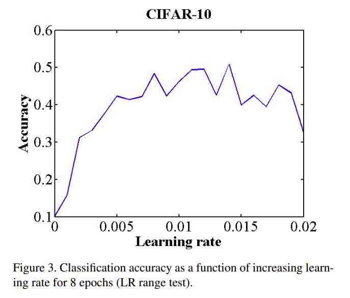
Figure 3 shows an example of making this type of run with the CIFAR-10 dataset, using the architecture and hyper-parameters provided by Caffe. One can see from Figure 3 that the model starts converging right away, so it is reasonable to set
base_lr = 0.001. Furthermore, above a learning rate of 0.006 the accuracy rise gets rough and eventually begins to drop so it is reasonable to setmax_lr = 0.006.
图3显示了使用Caffe实现的模型和超参数在CIFAR-10数据集上运行的示例。从图3可以看出,模型立即开始收敛,因此设置base_lr = 0.001是合理的。此外,在0.006学习率开始,准确度上升变得粗糙,并最终开始下降,因此设置max_lr = 0.006是合理的
Whenever one is starting with a new architecture or dataset, a single LR range test provides both a good LR value and a good range. Then one should compare runs with a fixed LR versus CLR with this range. Whichever wins can be used with confidence for the rest of one’s experiments.
无论何时从新的架构或数据集开始,单个LR范围测试都可以提供良好的LR值和良好的范围。然后在这个范围内比较固定LR和CLR的训练情况。使用效果更好的学习率方法用于后续的实验
根据损失值寻找最优学习率
参考:[译]如何找到一个好的学习率(learning rate)
上面论文提到的LR Range Test实现比较粗糙,文章How Do You Find A Good Learning Rate给出了一个更好的学习方法:比较平滑损失值(smoothed loss)和对数学习率(log LR)
平滑损失
设置一个非常低的学习率(比如
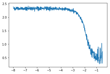
损失值在开始的时候组建下降,然后随着学习率的增大达到了最低点,最后开始快速上升
上图绘制比较粗糙,作者提供了一个平滑损失的计算方式。首先计算平均损失
其中
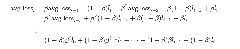
然后计算权重之和(这一步没理解,为啥可以撇开loss)

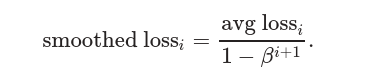
最后计算平滑损失:
对数学习率
在计算过程中,假定初始学习率为
如果使用
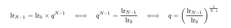
计算对数学习率如下:
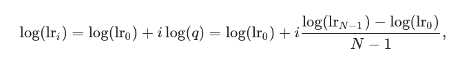
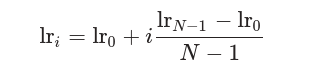
表示预设的最高学习率 表示预设的最低学习率 表示迭代次数
绘制
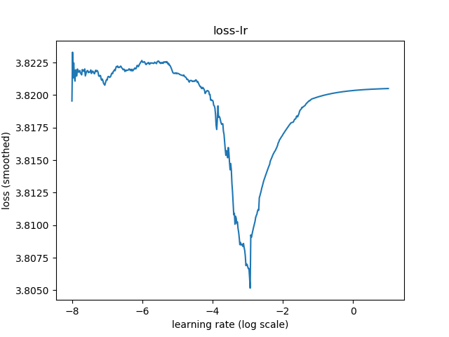
绘制平滑损失和学习率如下:
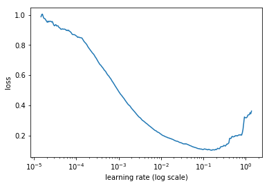
在绘制过程中为了防止损失值爆炸导致无法绘制,遵循以下原则:
从上图中,选择最大学习率为
PyTorch实现
作者提供了FastAI版本,当前使用PyTorch实现
1 | def find_lr(data_loader, model, criterion, optimizer, device, init_value=1e-8, final_value=10., beta=0.98): |
完整的测试代码参考:image-processing/py/lr
训练参数
- 模型:
SqueezeNet - 数据集:
CIFAR100 - 损失函数:
标签平滑正则化 - 优化器:
Adam - 批量大小:
96 - 学习率:最小学习率
1e-8,最高学习率10
最优学习率
执行py/lr/find_lr.py:
训练比对
根据学习率训练结果,设置3e-4作为最佳学习率;通常情况下,会使用1e-3作为最大学习率。执行py/lr/train.py,训练10轮结果如下:
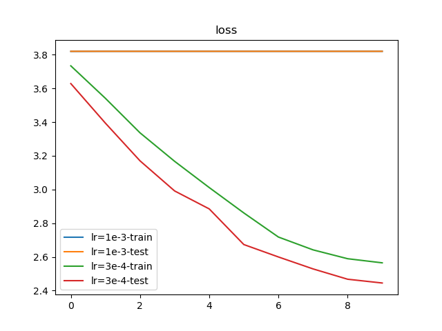
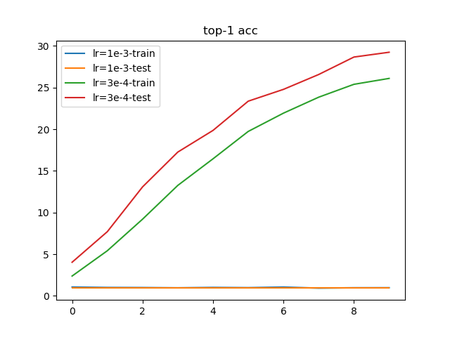
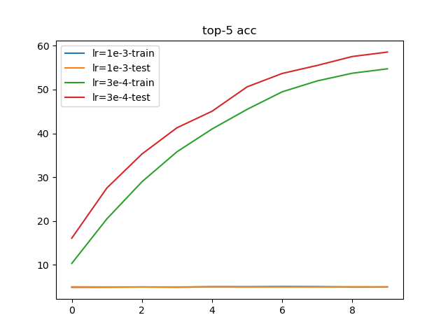
从训练结果上看,使用1e-3作为起始学习率会导致损失值完全不收敛;而使用3e-4作为起始学习率能够进行有效的训练