1
2
3
4
5
6
7
8
9
10
11
12
13
14
15
16
17
18
19
20
21
22
23
24
25
26
27
28
29
30
31
32
33
34
35
36
37
38
39
40
41
42
43
44
45
46
47
48
49
50
51
52
53
54
55
56
57
58
59
60
61
62
63
64
65
66
67
68
69
70
71
72
73
74
75
76
77
78
79
80
81
82
83
84
85
86
87
88
89
90
91
92
93
94
95
96
97
98
99
100
101
102
103
104
105
106
107
108
109
110
111
112
113
114
115
116
117
118
119
120
121
122
123
124
125
126
127
128
129
130
131
132
133
134
135
136
| # -*- coding: utf-8 -*-
"""
@author: zj
@file: multi-roc-nn.py
@time: 2020-01-11
"""
# -*- coding: utf-8 -*-
"""
@author: zj
@file: 2-roc.py
@time: 2020-01-10
"""
from mnist_reader import load_mnist
from nn_classifier import NN
import numpy as np
import matplotlib.pyplot as plt
from scipy import interp
from sklearn import datasets
from sklearn.model_selection import train_test_split
from sklearn.preprocessing import label_binarize
from sklearn.metrics import auc
from sklearn.metrics import roc_curve
from sklearn.metrics import roc_auc_score
def load_data():
    # Import some data to play with
    iris = datasets.load_iris()
    X = iris.data
    y = iris.target

    # shuffle and split training and test sets
    X_train, X_test, y_train, y_test = train_test_split(X, y, test_size=.5)

    return X_train, X_test, y_train, y_test
if __name__ == '__main__':
X_train, X_test, y_train, y_test = load_data()
n_classes = 3
# 数据标准化
x_train = X_train.astype(np.float64)
x_test = X_test.astype(np.float64)
mu = np.mean(x_train, axis=0)
var = np.var(x_train, axis=0)
eps = 1e-8
x_train = (x_train - mu) / np.sqrt(np.maximum(var, eps))
x_test = (x_test - mu) / np.sqrt(np.maximum(var, eps))
# 定义分类器,训练和预测
classifier = NN(None, input_dim=4, num_classes=3)
classifier.train(x_train, y_train, num_iters=100, batch_size=8, verbose=True)
res_labels, y_score = classifier.predict(x_test)
# print(y_score)
# Compute ROC curve and ROC area for each class
fpr = dict()
tpr = dict()
roc_auc = dict()
# Binarize the output 将类别标签二值化
y_test = label_binarize(y_test, classes=[0, 1, 2])
# one vs rest方式计算每个类别的TPR/FPR以及AUC
for i in range(n_classes):
fpr[i], tpr[i], _ = roc_curve(y_test[:, i], y_score[:, i])
roc_auc[i] = auc(fpr[i], tpr[i])
# Compute micro-average ROC curve and ROC area
# 微平均方式计算TPR/FPR,最后得到AUC
fpr["micro"], tpr["micro"], _ = roc_curve(y_test.ravel(), y_score.ravel())
roc_auc["micro"] = auc(fpr["micro"], tpr["micro"])
# 直接调用函数计算
micro_auc = roc_auc_score(y_test, y_score, average='micro')
lw = 2
# plt.figure()
# plt.plot(fpr[2], tpr[2], color='darkorange', lw=lw, label='ROC curve (area = %0.2f)' % roc_auc[2])
# plt.plot([0, 1], [0, 1], color='navy', lw=lw, linestyle='--')
# plt.xlim([0.0, 1.0])
# plt.ylim([0.0, 1.05])
# plt.xlabel('False Positive Rate')
# plt.ylabel('True Positive Rate')
# plt.title('Receiver operating characteristic example')
# plt.legend(loc="lower right")
# plt.show()
# First aggregate all false positive rates
all_fpr = np.unique(np.concatenate([fpr[i] for i in range(n_classes)]))
# Then interpolate all ROC curves at this points
mean_tpr = np.zeros_like(all_fpr)
for i in range(n_classes):
mean_tpr += interp(all_fpr, fpr[i], tpr[i])
# Finally average it and compute AUC
mean_tpr /= n_classes
fpr["macro"] = all_fpr
tpr["macro"] = mean_tpr
roc_auc["macro"] = auc(fpr["macro"], tpr["macro"])
# 直接调用函数计算
macro_auc = roc_auc_score(y_test, y_score, average='macro')
print(roc_auc)
print('micro auc:', micro_auc)
print('macro auc:', macro_auc)
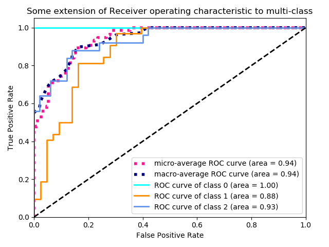
# Plot all ROC curves
plt.figure()
plt.plot(fpr["micro"], tpr["micro"],
label='micro-average ROC curve (area = {0:0.2f})'.format(roc_auc["micro"]),
color='deeppink', linestyle=':', linewidth=4)
plt.plot(fpr["macro"], tpr["macro"],
label='macro-average ROC curve (area = {0:0.2f})'.format(roc_auc["macro"]),
color='navy', linestyle=':', linewidth=4)
colors = ['aqua', 'darkorange', 'cornflowerblue']
for i, color in zip(range(n_classes), colors):
plt.plot(fpr[i], tpr[i], color=color, lw=lw,
label='ROC curve of class {0} (area = {1:0.2f})'.format(i, roc_auc[i]))
plt.plot([0, 1], [0, 1], 'k--', lw=lw)
plt.xlim([0.0, 1.0])
plt.ylim([0.0, 1.05])
plt.xlabel('False Positive Rate')
plt.ylabel('True Positive Rate')
plt.title('Some extension of Receiver operating characteristic to multi-class')
plt.legend(loc="lower right")
plt.show()
|