学习多分类任务的混淆矩阵计算,共有两种方式:
one VS restone VS one
one VS rest 指定其中一个类别为正样本,将其他类别统统归类为负样本,然后进行混淆矩阵的计算
python sklearn提供了实现函数:sklearn.metrics.multilabel_confusion_matrix
1 def multilabel_confusion_matrix(y_true, y_pred, sample_weight=None, labels=None, samplewise=False):
y_true:一维数组(仅输出正样本标签)或者多维矩阵(n_samples, n_outputs)y_pred:和y_true的格式一样labels:列表形式,指定正样本的顺序,否则函数将按排序顺序进行计算
该函数计算基于每个类别的混淆矩阵,输出大小为(n_outputs, 2, 2),每个混淆矩阵的排列如下:
示例 对3类任务进行计算,输入标签如下:
1 ['cat', 'ant', 'cat', 'cat', 'ant', 'bird']
预测标签如下:
1 ['ant', 'ant', 'cat', 'cat', 'ant', 'cat']
计算每类的混淆矩阵,并指定计算顺序:
1 res = multilabel_confusion_matrix(y_true, y_pred, labels=["ant", "bird", "cat"])
输出大小为(3, 2, 2)
1
2
3
4
5
6
7
8
[[[3 1] [0 2]] [[5 0] [1 0]] [[2 1] [1 2]]]
one VS one 在多分类任务中,还可以对每两个类别进行混淆矩阵的计算
python sklearn提供了实现函数:sklearn.metrics.confusion_matrix
1 def confusion_matrix(y_true, y_pred, labels=None, sample_weight=None):
y_true:一维数组,指定正样本y_pred:一维数组,输出预测标签labels:指定正样本顺序
函数返回一个(n_classes, n_classes)大小的混淆矩阵
示例 如果是二分类,其混淆矩阵排列为:
1
2
3
4
5
6
7
from sklearn.metrics import confusion_matrix if __name__ == '__main__': tn, fp, fn, tp = confusion_matrix([0, 1, 0, 1], [1, 1, 1, 0]).ravel() print(tn, fp, fn, tp) # 输出 0 2 1 1
如果是多分类,其输出如下:
1
2
3
4
5
6
7
8
9
10
11
from sklearn.metrics import confusion_matrix if __name__ == '__main__': y_true = ["cat", "ant", "cat", "cat", "ant", "bird"] y_pred = ["ant", "ant", "cat", "cat", "ant", "cat"] res = confusion_matrix(y_true, y_pred, labels=["ant", "bird", "cat"]) print(res) # 输出 [[2 0 0] [0 0 1] [1 0 2]]
点
点
利用混淆矩阵查看错误分类 利用one vs one的方式计算多分类任务,能够理清具体的错误分类场景
数据集 参考Fashion-MNIST数据集解析
分类器 参考神经网络分类器
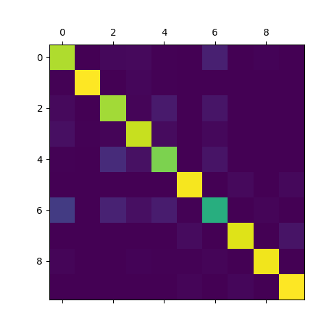
实现 1 2 3 4 5 6 7 8 9 10 11 12 13 14 15 16 17 18 19 20 21 22 23 24 25 26 27 28 29 30 31 32 33 34 35 36 37 38 39 40 41 42 43 44 45 46 # -*- coding: utf-8 -*- """ @author: zj @file: confusion-matrix.py @time: 2020-01-11 """ from nn_classifier import NN from mnist_reader import load_mnist import numpy as np import cv2 from sklearn.metrics import confusion_matrix import matplotlib.pyplot as plt def load_data(): path = "/home/zj/data/fashion-mnist/fashion-mnist/data/fashion/" train_images, train_labels = load_mnist(path, kind='train') test_images, test_labels = load_mnist(path, kind='t10k') return train_images, train_labels, test_images, test_labels if __name__ == '__main__': train_images, train_labels, test_images, test_labels = load_data() print(train_images.shape) print(train_labels.shape) x_train = train_images.astype(np.float64) x_test = test_images.astype(np.float64) mu = np.mean(x_train, axis=0) var = np.var(x_train, axis=0) eps = 1e-8 x_train = (x_train - mu) / np.sqrt(np.maximum(var, eps)) x_test = (x_test - mu) / np.sqrt(np.maximum(var, eps)) classifier = NN([100, 20], input_dim=28 * 28, num_classes=10) classifier.train(x_train, train_labels, verbose=True) y_pred = classifier.predict(x_test) cm = confusion_matrix(test_labels, y_pred) print(cm) plt.matshow(cm) plt.show()
使用神经网络分类Fashion-MNIST,结果如下:
1
2
3
4
5
6
7
8
9
10
[[852 1 21 25 4 0 86 0 11 0] [ 7 967 3 16 5 0 1 0 1 0] [ 25 1 833 12 70 1 55 0 3 0] [ 38 5 14 888 30 2 20 0 3 0] [ 6 1 118 44 776 1 52 0 2 0] [ 0 0 0 0 1 955 0 23 2 19] [167 1 93 38 75 4 608 0 14 0] [ 0 0 0 0 0 28 0 921 0 51] [ 12 2 2 8 5 7 12 3 948 1] [ 0 0 1 0 0 14 1 16 0 968]]
从混淆矩阵中可以发现,标签0(就是T恤)最容易错误分类为标签6(就是衬衫);标签4(就是外套)最容易错误分类为标签2(就是套衫)
相关阅读