ROC曲线(receiver operating characteristic curve,受试者工作特征曲线)是一个二维图,用于说明分类器在不同阈值下的分类能力
本文通过ROC曲线评价二元分类器
TPR
TPR(true positive rate)指的是检测为真的正样本占实际正样本集的比率,称为真阳性率,也称为召回率(recall rate)、敏感度(sensitivity),检测率(probability of detection)。计算公式如下:
FPR
FPR(false positive rate)指的是检测为假的负样本占实际负样本集的比率,称为假阳性率,也称为误报率(probability of false alarm)。计算公式如下:
ROC curve
ROC curve全称是受试者工作特征曲线(receiver operating characteristic curve),它是一个二维曲线图,用于表明分类器的检测性能
其y轴表示TPR,x轴表示FPR。通过在不同阈值条件下计算(FPR, TPR)数据对,绘制得到ROC曲线

ROC描述了收益(true positive)和成本(false positive)之间的权衡。由上图可知
- 最好的预测结果发生在左上角
(0,1),此时所有预测为真的样本均为实际正样本,没有正样本被预测为假
- 对角线表示的是随机猜测(
random guess)的结果,对角线上方的坐标点表示分类器的检测结果比随机猜测好
所以离左上角越近,表示预测效果越好,此时分类器的性能更佳
如何通过ROC曲线判断分类器性能 - AUC
AUC(Area under curve)指的是ROC曲线下的面积。其表示概率值:当随机给定一个正样本和一个负样本,分类器输出该正样本为正的概率值比分类器输出该负样本为正的概率值要大的可能性
AUC越大,表明分类器性能越强
python实现
sklean库提供了多个函数用于ROC/AUC的计算,参考3.3.2.14. Receiver operating characteristic (ROC)
roc_curve
1
2
| def roc_curve(y_true, y_score, pos_label=None, sample_weight=None,
drop_intermediate=True):
|
y_true:一维数组形式,表示样本标签。如果不是{-1,1}或者{0,1}的格式,那么参数pos_label需要显式设定y_score:一维数组形式,表示目标成绩。可以是对正样本的概率估计/置信度pos_label:指明正样本所属标签。如果y_true是{-1,1}或{0,1}格式,那么pos_label默认为1
1
2
3
4
5
6
7
8
9
10
11
12
13
14
| import numpy as np
from sklearn.metrics import roc_curve
y = np.array([1, 1, 2, 2])
scores = np.array([0.1, 0.4, 0.35, 0.8])
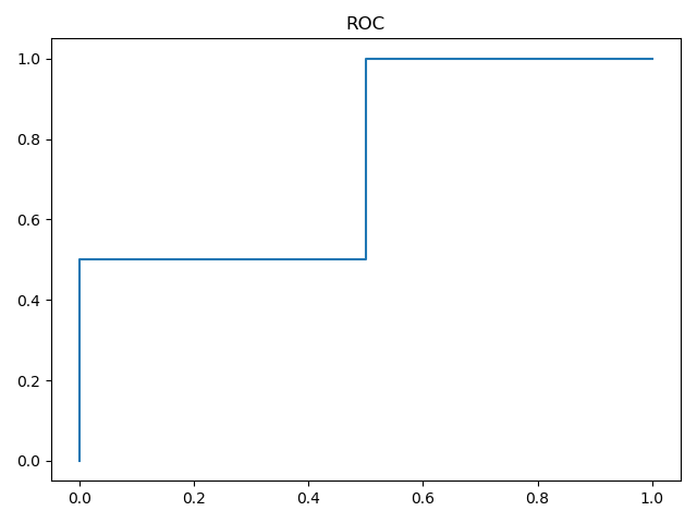
fpr, tpr, thresholds = roc_curve(y, scores, pos_label=2)
fig = plt.figure()
plt.plot(fpr, tpr, label='ROC')
plt.show()
// 输出
[0. 0. 0.5 0.5 1. ] # FPR
[0. 0.5 0.5 1. 1. ] # TPR
[1.8 0.8 0.4 0.35 0.1 ] # thresholds
|
返回的是FPR、TPR和阈值数组,FPR和TPR中每个坐标的值表示利用thresholds数组同样下标的阈值所得到的真阳性率和假阳性率
roc_auc_score/auc
1
2
| def roc_auc_score(y_true, y_score, average="macro", sample_weight=None,
max_fpr=None):
|
y_true:格式为[n_samples]或者[n_samples, n_classes]y_score:格式为[n_samples]或者[n_samples, n_classes]
返回的是AUC的值
1
| def auc(x, y, reorder='deprecated'):
|
利用roc_curve计算得到FPR和TPR后,就可以输入到auc计算AUC大小
1
2
3
4
5
6
7
8
| from sklearn.metrics import roc_auc_score
from sklearn.metrics import auc
print(roc_auc_score(y, scores))
print(auc(fpr, tpr))
# 输出
0.75
0.75
|
如何计算最佳阈值
通过ROC图可知,TPR越大越好,FPR越小越好,所以只要能够得到不同阈值条件下的TPR和FPR,计算之间的差值,结果值最大的就是最佳阈值
1
2
| thresh = thresholds[np.argmax(tpr - fpr)]
print(thresh)
|
示例
数据集
使用数据集Fashion-MNIST中的Sneaker(运动鞋,编号为7)和Ankle boot(短靴,编号为9)类别进行训练和测试
1
2
3
4
5
6
7
8
9
10
11
12
13
14
15
16
17
18
19
20
21
| from mnist_reader import load_mnist
def get_two_cate():
path = "/home/zj/data/fashion-mnist/fashion-mnist/data/fashion/"
train_images, train_labels = load_mnist(path, kind='train')
test_images, test_labels = load_mnist(path, kind='t10k')
num_train_seven = np.sum(train_labels == 7)
num_train_nine = np.sum(train_labels == 9)
print(num_train_seven, num_train_nine)
num_test_seven = np.sum(test_labels == 7)
num_test_nine = np.sum(test_labels == 9)
print(num_test_seven, num_test_nine)
x_train = train_images[(train_labels == 7) + (train_labels == 9)]
y_train = train_labels[(train_labels == 7) + (train_labels == 9)]
x_test = test_images[(test_labels == 7) + (test_labels == 9)]
y_test = test_labels[(test_labels == 7) + (test_labels == 9)]
return x_train, (y_train == 9) + 0, x_test, (y_test == 9) + 0
|
- 训练集个数为
12000,每类样本各6000
- 测试集个数为
2000,每类样本各1000
正确率
通过计算正确率来判断通过ROC曲线得到的阈值的效果
1
2
3
4
5
| def compute_accuracy(y, y_pred):
num = y.shape[0]
num_correct = np.sum(y_pred == y)
acc = float(num_correct) / num
return acc
|
分类器
使用逻辑回归分类器进行二分类ROC曲线的计算。对于二分类逻辑回归而言,对于每个检测样本,计算得到一个数值(取值为(0,1)),一般使用阈值0.5进行判断
在本次实验中,修改预测函数,返回阈值0.5的检测结果以及样本的置信度
1
2
3
4
5
| def predict(self, X):
scores = self.logistic_regression(X)
y_pred = (scores > 0.5).astype(np.uint8)
return y_pred, scores
|
计算
实现如下:
1
2
3
4
5
6
7
8
9
10
11
12
13
14
15
16
17
18
19
20
21
22
23
24
25
26
27
28
29
30
31
32
33
34
35
36
37
38
39
40
41
42
| if __name__ == '__main__':
# 获取二类样本集
train_images, train_labels, test_images, test_labels = get_two_cate()
print(train_images.shape)
print(test_images.shape)
# cv2.imshow('img', train_images[100].reshape(28, -1))
# cv2.waitKey(0)
# 数据标准化
x_train = train_images.astype(np.float64)
x_test = test_images.astype(np.float64)
mu = np.mean(x_train, axis=0)
var = np.var(x_train, axis=0)
eps = 1e-8
x_train = (x_train - mu) / np.sqrt(np.maximum(var, eps))
x_test = (x_test - mu) / np.sqrt(np.maximum(var, eps))
# 定义逻辑回归分类器,训练并进行预测
classifier = LogisticClassifier()
classifier.train(x_train, train_labels)
res_labels, scores = classifier.predict(x_test)
# 计算阈值0.5时的准确率
acc = compute_accuracy(test_labels, res_labels)
print(acc)
# 计算fpr/trp/阈值
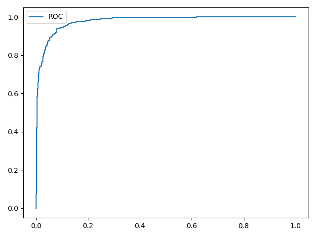
fpr, tpr, thresholds = roc_curve(test_labels, scores, pos_label=1)
fig = plt.figure()
plt.plot(fpr, tpr, label='ROC')
plt.legend()
plt.show()
# 计算最佳阈值
thresh = thresholds[np.argmax(tpr - fpr)]
print(thresh)
# 计算最佳阈值下的准确率
y_pred = (scores > thresh).astype(np.uint8)
acc = compute_accuracy(test_labels, y_pred)
print(acc)
|
结果如下:
1
2
3
4
5
| (12000, 784)
(2000, 784)
0.92
0.4644471941592551
0.9285
|
由输出结果可知,最佳阈值为0.4644,最终得到的准确率提升了0.75%
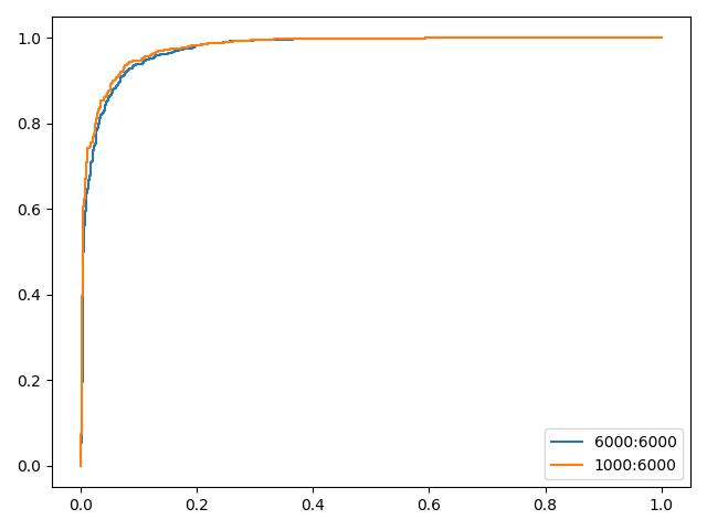
类别不平衡
设置类别Sneaker的训练个数为1000,同时保持Ankle boot的训练个数为6000,训练后绘制ROC曲线
1
2
3
4
5
6
7
8
9
10
11
12
13
14
15
16
17
18
19
20
21
22
23
24
| def get_two_cate():
path = "/home/zj/data/fashion-mnist/fashion-mnist/data/fashion/"
train_images, train_labels = load_mnist(path, kind='train')
test_images, test_labels = load_mnist(path, kind='t10k')
num_train_seven = np.sum(train_labels == 7)
num_train_nine = np.sum(train_labels == 9)
print(num_train_seven, num_train_nine)
num_test_seven = np.sum(test_labels == 7)
num_test_nine = np.sum(test_labels == 9)
print(num_test_seven, num_test_nine)
x_train_0 = train_images[(train_labels == 7)]
x_train_1 = train_images[(train_labels == 9)]
y_train_0 = train_labels[(train_labels == 7)]
y_train_1 = train_labels[(train_labels == 9)]
x_train = np.vstack((x_train_0[:1000], x_train_1))
y_train = np.concatenate((y_train_0[:1000], y_train_1))
x_test = test_images[(test_labels == 7) + (test_labels == 9)]
y_test = test_labels[(test_labels == 7) + (test_labels == 9)]
return x_train, (y_train == 9) + 0, x_test, (y_test == 9) + 0
|
计算结果如下:

1
2
3
4
5
6
7
| (7000, 784)
(2000, 784)
[0 0 0 ... 0 1 1]
[1 0 0 ... 0 1 1]
0.867 # 阈值0.5的正确率
0.36547217942403787
0.9235 # 阈值0.3655的正确率
|
对比实验结果,ROC曲线能够有效验证类别样本数不平衡时的分类器性能
小结
ROC曲线图能够不受类别数不平衡的影响,简单、直观的展示不同阈值下的分类器性能
相关阅读